R E S E A R C H
Open Access
A gradient-adaptive lattice-based
complex adaptive notch filter
Rui Zhu, Feiran Yang and Jun Yang
*Abstract
This paper presents a new complex adaptive notch filter to estimate and track the frequency of a complex sinusoidal signal. The gradient-adaptive lattice structure instead of the traditional gradient one is adopted to accelerate the convergence rate. It is proved that the proposed algorithm results in unbiased estimations by using the ordinary differential equation approach. The closed-form expressions for the steady-state mean square error and the upper bound of step size are also derived. Simulations are conducted to validate the theoretical analysis and demonstrate that the proposed method generates considerably better convergence rates and tracking properties than existing methods, particularly in low signal-to-noise ratio environments.
Keywords: Frequency tracking, Adaptive notch filter, Gradient-adaptive lattice, Steady-state mean square error
1 Introduction
The adaptive notch filter (ANF) is an efficient frequency estimation and tracking technique that is utilised in a wide variety of applications, such as communication systems, biomedical engineering and radar systems [1–12]. The complex ANF (CANF) has recently gained much atten-tion [13–20]. A direct-form poles and zeros constrained CANF was first developed in [13] with a modified Gauss-Newton algorithm. A recursive least square (RLS)-based Steiglitz-McBride (RLS-SM) algorithm was also estab-lished to accelerate the convergence rate [14]. However, both algorithms are computationally complicated and can result in biased estimations.
To address this problem, numerous efficient and unbi-ased least mean square (LMS)-bunbi-ased algorithms have been developed, such as the complex plain gradient (CPG) [15], modified CPG (MCPG) [16], lattice-form CANF (LCANF) [17], and arctangent-based algorithms [18]. However, all these LMS-based algorithms generate a lower convergence rate than the RLS-based algorithms do. Moreover, the upper bound of the step size in LMS-based methods must be maintained within a limited range to ensure stability; this range depends on the eigen-value of the correlation matrix of the input signal. These
*Correspondence: [email protected]
The State Key Laboratory of Acoustics and the Key Laboratory of Noise and Vibration Research, Institute of Acoustics, Chinese Academy of Sciences, 21, Beisihuanxilu Road, 100190 Beijing, China
drawbacks limit the practical applications of LMS-based algorithms.
Several normalized LMS (NLMS)-based CANF algo-rithms were established, including the normalized CPG (NCPG) algorithm [19] and the improved simplified lat-tice complex algorithm [20]. However, the former may be unstable in low signal-to-noise ratio (SNR) condi-tions, and the latter can only be used to estimate positive instantaneous frequency.
In this paper, we develop a new CANF system based on the lattice algorithm [21]. Instead of the traditional gra-dient estimation filter, we proposed a normalized lattice predictor that makes both forward and backward predic-tions. This scheme reduces computational complexity and enhances the robustness to noise influence. Furthermore, convergence rate is improved significantly when com-pared with conventional gradient-based or nongradient-based methods without sacrificing tracking property.
A classic ordinary differential equation (ODE) method is applied to confirm the unbiasedness of the proposed algo-rithm. In addition, theoretical analyses are conducted on the stable range of the step size and the steady-state mean square error (MSE) under different conditions. Computer simulations are conducted to confirm the validity of the theoretical analysis results and the effectiveness of the proposed algorithm.
The following notations are adopted throughout this paper.jdenotes square root of minus one. ln[·] denotes
the principal branch of the complex natural logarithm
function and Im{·} means taking the imaginary part of
a complex value. Z{·} and E{·} denote the z-transform
operator and statistical expectation operator, respectively.
δ(·) represents the Dirac function. Asterisk∗denotes a
complex conjugate and⊗is the convolution operator.
2 Filter structure and adaptive algorithm
We consider the following noisy complex sinusoidal input
signal x(n) with amplitude A, frequency ω0 and initial
phaseφ0:
x(n)=Aej(ω0n+φ0)+v(n), (1)
whereφ0is uniformly distributed over [ 0, 2π)andv(n)=
vr(n)+jvi(n)is assumed to be a zero-mean white complex Gaussian noise process. It is assumedvr(n)andvi(n)are uncorrelated zero-mean real white noise processes with identical variances. The first-order, pole-zero-constrained CANF with the following transfer function is widely used
to estimate frequency ω0: H(z) = 1−e
jθz−1
1−αejθz−1 where θ
is the notch frequency and α represents the pole-zero
constrained factor and determines the notch filter’s 3-dB attenuation bandwidth. The pole can remain in the unit circle by restricting the value ofα.
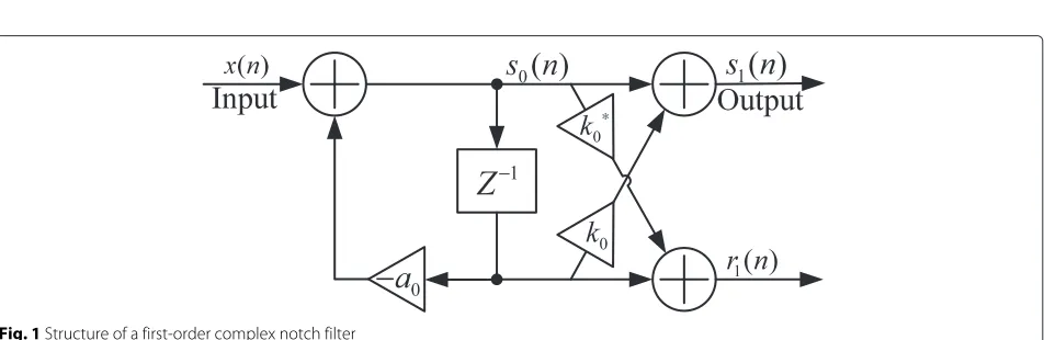
We now propose a new structure to implement the complex notch filter. As shown in Fig. 1, the input sig-nalx(n)is first processed by an all-pole prefilterHp(z) = 1/D(z) = 1/(1 + a0z−1) to obtain s0(n), where a0 is
the coefficient of the all-pole filter. Then, a lattice pre-dictor is employed to identify the forward and backward prediction errorss1(n)andr1(n), respectively. The
trans-form functions froms1(n)andr1(n)tos0(n)are given by
Hf(z) = N(z) = 1+k0z−1andHb(z) = z−1N∗(z) =
k0∗+z−1(k0being the reflection coefficient of the lattice
filter). To acquire the desired pole-zero constrained notch filter, the following relations must be satisfied:
k0= −ejθ, (2)
a0=αk0. (3)
Thus,θcan be computed asθ =Im{ln[−k0]}.
At this point, a normalized stochastic gradient algo-rithm is derived to update the reflection coefficientk0. We
consider the following cost function:
Jfb= 1 2E
|s1(n)|2+ |r1(n)|2
, (4)
We replace cost functionJfbwith its instantaneous esti-mation, i.e.,
ˆ Jfb=
1 2
|s1(n)|2+ |r1(n)|2
. (5)
By taking the derivative ofJˆfbwith respect toθ(n), we obtain
∇ˆJfb=
dˆJfb(n)
dk0(n)
dk0(n)
dθ(n) = −Im{s1(n)s0
∗(n)}. (6)
Considering thatθ(n) is real, the adaptation equation can be written as
θ(n+1)=θ(n)+μ·Im{s1(n)s0∗(n)}/ξ(n), (7)
whereμis the step size and the normalized signalξ(n)can be recursively calculated as
ξ(n)=ρξ(n−1)+(1−ρ)s0∗(n)s0(n), (8)
whereρdenotes the smoothing factor.
Table 1 shows the computational complexities of the proposed algorithm and of four conventional methods [14, 16, 17, 19]. Note that the complexity of the proposed algorithm is comparable to that of LMS-based meth-ods and lower than that of NLMS-based and RLS-based algorithms.
3 Convergence analysis
We now use the ODE approach to analyse the convergence properties of the adaptive algorithm, which has been applied to analyse several other ANF algorithms [17, 22]. Assuming that the adaptation is sufficiently slow and the input signal is stationary, the associated ODEs for the proposed adaptive algorithm can be expressed as
Table 1Complexities of the proposed algorithm and of four associated ordinary differential equation of the proposed adaptive algorithm, according to [23], θ(n) will always converge to the stationary point of Eq. 9 without excep-tion, and this stationary point must satisfy ddτθ(τ) = 0.
ξ(τ)is always positive; therefore, the stationary point of
θ(n) converges to a solution of equation f(θ(τ)) = 0.
Based on Eq. 11, θ = ω0 is the sole stationary point
over one period of the function. To confirm that the sta-tionary point is stable, we choose a Lyapunov function
L(τ)=[ω0−θ(τ)]2.L(τ)≥0 for allτ. Meanwhile,
is maintained for allθ(τ)=ω0. This equation implies that
L(τ)is a decreasing function of τ for|ω0−θ(τ)| < π.
Thus, it is proved that θ(n) can always converge to the expected frequencyω0[23].
Now, we would like to compute the upper bound of step sizeμ. Taking the expectation on both sides of Eq. 7, we obtain
Taking ensemble expectations on both sides and assum-ing thats0(n)is wide-sense stationary, we have
lim
In each step, we consider that [24]
ξ(n)=rS0(0)+ξ(n), (17)
whereξ(n) is the zero-mean stochastic error sequence
that is independent of the input signal. By applying Eq. 17 and disregarding the second-order error, we obtain
1
By substituting Eqs. 11, 16, and 18 into Eq. 13, we get
¯
Considering the approximations sin(θ−ω0)¯
ω0− ¯θ(n+1)=
(0, 2], which is independent of the input.
4 Steady-state MSE analysis
In this section, a PSD-based method [19, 25] is exploited to derive the accurate expressions for the steady-state MSE of the estimated frequency. As discussed in the previous section, the estimated frequency can converge to an unbiased value, i.e., lim
n→∞ θ(n) = ω0.
Defin-ing that θ(n) = θ(n) − ω0, we obtain the following
two approximations: lim
n→∞ sin(θ(n)) ≈ θ(n) and
lim
n→∞ cos(θ(n)) ≈ 1. Then, the steady-state transfer function froms1(n)ands0(n)tox(n)can be written as:
The input signalx(n)in Eq. 1 is assumed to be composed of a single frequency part and Gaussian white noise. Thus, the steady-state outputss1(n)ands0(n)can be expressed
as:
By substituting Eqs. 23 and 24 into Eq. 7, the adaptive update equation can be rewritten as
θ(n+1)=θ(n)+ ¯μ·
Substituting Eqs. 25 and 26 into Eq. 31 yields
u3(n)≈ −
A2θ(n)
(1−α)2. (33)
Meanwhile, Eq. 32 can be rearranged as
u4(n)≈Im(ns0
Assuming α is close to unity or the SNR is sufficient
large, it stands that u3(n)
Therefore, by subtractingω0from both sides of Eq. 27
and assuming u(n) = u1(n) + u2(n) and β = 1 −
Hence, the MSE of the estimated frequency can be expressed as [26]: autocorrelation sequence ofu(n)and can be calculated as:
ru(l) = E{u(k+l)u∗(k)}
= ru1(l)+ru2(l)+2ru1u2(l), (39)
where
ru2(l)=E[u2(n+l)u2(n)] , (41)
and
ru1u2(l)=E[u1(n+l)u2(n)] . (42)
ThusRu(z)in Eq. 38 can be divided into three parts:
Ru(z) = Z{ru(l)}
and then Eq. 40 can be rearranged as:
ru1(l)=E[u1(n+l)u1(n)]= −
By using the results in Appendix A and considering that
ss0(n)andns1(n)are uncorrelated, we can rewrite Eqs. 46,
Substituting Eqs. 50, 51, 52, and 53 into Eq. 45, we get
ru1(l)= Substituting Eq. 57 into Eq. 56 yields
ru1(l)=
The z-transform of both sides of Eq. 58 can be expressed as:
following results (see Appendix B for details)
Ru2(z)=
Substituting Eqs. 61, 62, and 63 into Eq. 38, finally we get
Eθ(n)2= μ¯ Equation 64 indicates that the estimated MSE is inde-pendent of input frequencyω0and smooth factorρ.
5 Simulation results
Computer simulations are conducted to confirm the effec-tiveness of the proposed algorithm and the validity of the theoretical analysis results.
5.1 Performance comparisons
fixed frequency input and a quadratic chirp input. The input signal takes the form x(n) = ej(ϕ(n)+θ0) + v(n),
where ϕ(n) is the instantaneous phase. The parameters
are adjusted to establish an equal steady-state MSE and an equal notch bandwidth for all the algorithms. The initial notch frequency value is set to zero for all the methods.
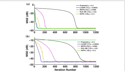
Figure 2 presents the MSE curves of five algorithms
with a fixed frequencyϕ(n) = 0.4πnat SNR =10 and
0 dB, respectively. Note that the proposed algorithm out-performs the other four algorithms. The NCPG algorithm achieves the similar convergence rate as the proposed algorithm at SNR = 10 dB while the former diverges at SNR = 0 dB. This indicates that the proposed algorithm is robust even at very low SNR conditions.
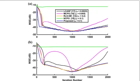
Figure 3 presents the tracking rate of the five algorithms with a quadratic chirp input signal: ϕ(n) = Ac(φ1n +
φ2n2+φ3n3), whereφ1 = −π/4,φ2 = π/2×10−3and
φ3 = −π/6×10−6. ParameterAcis adopted to control the value of chirp rate. For this case, the desired true fre-quency can be obtained by∂ϕ(n)/∂n = Ac(φ1+2φ2n+
3φ3n). Figure 3a depicts the tracking MSE obtained when
Ac = 1, and Fig. 3b presents the MSE with an increased
chirp rate: Ac = 2. The results imply that under the
non-stationary case, the proposed method can achieve faster convergence speed than all the other four algo-rithms. When tracking speed is concerned, we see that the
RLS-SM method and the proposed method can maintain an equally small MSE than the other three methods espe-cially at the high chirp rate part. We checked each of the learning curves of the NCPG algorithm and found that this algorithm even diverges in some runs.
5.2 Simulations of steady-state estimation MSE
In the following four simulations, the simulated steady-state MSE of the proposed algorithm is compared with the theoretical results in Eq. 64 with different input frequency
ω0, SNR, pole radius α and step size μ. The simulation
results are obtained by averaging over 500 trials.
Figure 4 displays the comparison of the theoretical and
simulated steady-state MSEs versus signal frequencyω0
under two different SNRs (SNR = 60 and 10 dB). The curves show that the theoretical MSEs can predict the simulated MSEs precisely, and the steady-state MSEs are
independent of input frequency ω0. We also see that a
higher SNR leads to a larger MSE.
Figure 5 exhibits the comparison of the theoretical and simulated steady-state MSEs versus SNR under two
dif-ferent parameter settings: (1)α = 0.9,μ = 0.8 and (2)
α = 0.98,μ = 0.1. The proposed approach predicts
the MSEs well, although some discrepancies are observed
with α = 0.9,μ = 0.8. That is because the CANF can
hardly converge when the SNR is very low.
0 200 400 600 800 1000 1200
−60 −40 −20 0
MSE (dB)
Proposed (μ = 0.1) LCANF [17] (μ = 0.0023) MCPG [16] (μ = 0.009) RLS−SM [14] (κ = 0.2) NCPG [19] (μ = 0.1)
0 200 400 600 800 1000 1200
−50 −40 −30 −20 −10
Iteration Number
MSE (dB)
Proposed (μ = 0.1) LCANF [17] (μ = 0.0023) MCPG [16] (μ = 0.005) RLS−SM [14] (κ = 0.2) NCPG [19] (μ = 0.1)
(a)
(b)
Fig. 3Comparison of the tracking behaviors for a quadratic chirp input under two different chirp rates (α= 0.9, SNR = 0 dB, and 1000 runs):a comparison of MSEs whenAc=1 andbcomparison of MSEs whenAc=2
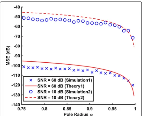
Figure 6 illustrates the comparison of the theoretical and simulated steady-state MSEs versus pole radiusα. Whenα decreases, the MSEs increase and the mismatch between the theoretical and simulated steady-state MSEs is some-what large. It is because Eq. 36 is derived on the basis of the assumption thatαis close to unity. Whenαis small,
Normalized Frequency
-1 -0.5 0 0.5 1
MSE (dB)
-100 -90 -80 -70 -60 -50 -40 -30
SNR = 60 dB (Simulation1) SNR = 60 dB (Theory1) SNR = 10 dB (Simulation2) SNR = 10 dB (Theory2)
Fig. 4Comparison of the theoretical and simulated steady-state MSEs versus signal frequencyω0at SNR = 60 dB and 10 dB (α=0.9 and μ=0.8)
the assumption does not hold. This explains the mismatch in Fig. 6. This finding implies that the theoretical MSE remains valid whenαis close to unity.
As shown in Fig. 7, the theoretical MSEs can predict the simulated steady-state MSEs well particularly forμ <
1.8 but the mismatch occurs whenμapproaches the up
Fig. 6Comparison of the theoretical and simulated steady-state MSEs versus pole radiusα(ω0= 0.2π,μ= 0.1, and 500 runs): (1) SNR = 60 dB and (2) SNR = 10 dB
boundary of the step size. Moreover, it is noted that a large step size yields a large MSE.
6 Conclusions
This paper has presented a complex adaptive notch fil-ter based on the gradient-adaptive lattice approach. The new algorithm is computationally efficient and can pro-vide an unbiased estimation. The closed-form expressions for the steady-state MSE and the upper bound of step size have been worked out. Simulation results demon-strate that (1) the proposed algorithm can achieve faster convergence rate than the traditional methods particularly
Fig. 7Comparison of the theoretical and simulated steady-state MSEs versus step sizeμ. (ω0= 0.2π,α= 0.95, and 500 runs): (1) SNR = 60 dB and (2) SNR = 10 dB
in the low SNR conditions and (2) theoretical analysis of the proposed algorithm is in good agreement with computer simulation results. By cascading the proposed first-order gradient-adaptive lattice filters, the algorithm can be extended to handle complex signal with mul-tiple sinusoids, which will be the focus of our further research.
Appendix A
Given complex sequencesf(n)andg(n), we define a new
functionζfg(l)as
ζfg(l)=E
f(n+l)g(n). (65)
Thus, for the input signalx(n)defined in Eq. 1, we have
ζxx(l) = E{x(n+l)x(n)} = A2ejω0lE
ej2(ω0n+φ0)
+ζvv(l). (66)
Given thatφ0is uniformly distributed over [ 0, 2π), we
haveE{ej2(ω0n+φ0)} =0.v(n) =vr(n)+jvi(n)is assumed to be a zero-mean white complex Gaussian noise process where vr(n) and vi(n) are uncorrelated zero-mean real white noise processes with identical variances. Therefore, we have the following relations:
rvr(l)=
σ2
v
2 δ(l), (67)
rvi(l)=
σ2
v
2 δ(l), (68)
rvrvi(l)=rvivr(l)=0, (69)
where rvr(l) andrvi(l)are the autocorrelation sequences
of vr(n) and vi(n), respectively. rvrvi(l) is the
cross-correlation sequence ofvr(n)andvi(n). Consequently, we obtain
ζvv(l) = E[v(n+l)v(n)]
= rvr(l)−rvi(l)+2jrvrvi(l)
= 0. (70)
Substituting Eq. 70 into Eq. 66, we get
ζxx(l)=0. (71)
ζxy(l) = E[x(n+l)y(n)]
Substituting Eq. 72 into Eq. 73 and considering Eq. 71, we get
ζyy(l)=h(−l)⊗h(l)⊗ζxx(l)=0 (74) By using Eq. 74, it is clear that
E{y(n)2} =ζyy(0)=0. (75)
and then Eq. 41 can be rearranged as:
ru2(l)=E[u2(n+l)u2(n)]= −
stationary processes and utilising the Gaussian moment factoring theorem [27], we get
q1(l)=cum(ns0
∗(n+l),n
s1(n+l)
,ns0∗(n),ns1(n))+rns1ns0(−l)rns1ns0(l)
+rns1ns0(0)rns1ns0(0)+ζn∗s0n∗s0(l)ζns1ns1(l), (82)
where cum(·)denotes high order cumulants of the
com-plex random variables. We adopt the widely used inde-pendence assumption [28], which tells that the present sample is independent of the past samples. Thus, we have cum(ns0∗(n+l),ns1(n+l),ns0∗(n),ns1(n))=0. And,
fur-the same method, we get
q2(l) = rns0ns1(0)rns0ns1(0)
Substituting Eqs. 83, 84, 85 and 86 into Eq. 77, we get
whereRn(z)=σv2andHs1(z)=
1+k0z−1
1+αk0z−1. Sincerns1(l)is a
two-sided sequence with the region of convergence given by|k0|/α >|z|> α|k0|, the inverse z-transform ofRns1(z)
whereu(l)denotes the unit step sequence. Using the same
method, we have
Substituting Eqs. 89, 90, 91, and 92 into 87, and taking the z-transform on both sides we have
Ru2(z)=Z{ru2(l)} = σ4
v
2(1−α2). (93)
Substituting Eqs. 44 and 76 into Eq. 42 and considering thatss0(n)is uncorrelated withns1(n)andns0(n), we have
Sincess0(n)is a zero-mean stationary process, it holds
thatru1u2(l)=0. Thus we get
Ru1u2(z)=Z{ru1u2(l)} =0. (95)
Acknowledgements
This work is supported by Strategic Priority Research Program of the Chinese Academy of Sciences under Grants XDA06040501, and in part by the National Science Fund of China under Grant 61501449. We thank the reviewers for their constructive comments and suggestions.
Competing interests
The authors declare that they have no competing interests.
Received: 9 January 2016 Accepted: 29 June 2016
References
1. L-M Li, LB Milstein, Rejection of pulsed cw interference in pn spread-spectrum systems using complex adaptive filters. IEEE Trans. Comm.COM-31, 10–20 (1983)
2. D Borio, L Camoriano, LL Presti, Two-pole and multi-pole notch filters: a computationally effective solution for GNSS interference detection and mitigation. IEEE Syst. J.2(1), 38–47 (2008)
3. RM Ramli, AOA Noor, SA Samad, A review of adaptive line enhancers for noise cancellation. Aust. J. Basic Appl. Sci.6(6), 337–352 (2012) 4. R Zhu, FR Yang, J Yang, in21st Int. Congress on Sound and Vibration 2014
(ICSV 2014). A variable coefficients adaptive IIR notch filter for bass enhancement (International Institute of Acoustics and Vibrations (IIAV), USA, 2014)
5. SW Kim, YC Park, YS Seo, DH Youn, A robust high-order lattice adaptive notch filter and its application to narrowband noise cancellation. EURASIP J. Adv. Signal Process.2014(1), 1–12 (2014)
6. A Nehorai, A minimal parameter adaptive notch filter with constrained poles and zeros. IEEE Trans. Acoust. Speech Signal Process.ASSP-33(8), 983–996 (1985)
7. NI Choi, CH Choi, SU Lee, Adaptive line enhancement using an IIR lattice notch filter. IEEE Trans. Acoust. Speech Signal Process.37(4), 585–589 (1989)
8. T Kwan, K Martin, Adaptive detection and enhancement of multiple sinusoids using a cascade IIR filter. IEEE Trans. Circ. Syst.36(7), 937–947 (1989)
9. PA Regalia, An improved lattice-based adaptive IIR notch filter. IEEE Trans. Signal Process.39, 2124–2128 (1991)
10. Y Xiao, L Ma, K Khorasani, A Ikuta, Statistical performance of the memoryless nonlinear gradient algorithm for the constrained adaptive IIR notch filter. IEEE Trans. Circ. Syst. I.52(8), 1691–1702 (2005)
11. J Zhou, inProc. Inst. Elect. Eng., Vis., Image Signal Process. Simplified adaptive algorithm for constrained notch filters with guaranteed stability, vol. 153 (The Institution of Engineering and Technology (IET), UK, 2006), pp. 574–580
12. L Tan, J Jiang, L Wang, Pole-radius-varying iir notch filter with transient suppression. IEEE Trans. Instrum. Meas.61(6), 1684–1691 (2012) 13. SC Pei, CC Tseng, Complex adaptive IIR notch filter algorithm and its
applications. IEEE Trans. Circ. Syst. II.41(2), 158–163 (1994) 14. Y Liu, TI Laakso, PSR Diniz, inProc. 2001 Finnish Signal Process. Symp.
(FINSIG01). A complex adaptive notch filter based on the Steiglitz-Mcbride method (Helsinki University of Technology, Finland, 2001), pp. 5–8 15. S Noshimura, HY Jiang, inProc. IEEE Asia Pacific Conf. Circuits and Systems.
Gradient-based complex adaptive IIR notch filters for frequency estimation (Institute of Electrical and Electronics Engineers (IEEE), USA, 1996), pp. 235–238
16. A Nosan, R Punchalard, A complex adaptive notch filter using modified gradient algorithm. Signal Process.92(6), 1508–1514 (2012)
17. PA Regalia, A complex adaptive notch filter. IEEE Signal Process. Lett.
17(11), 937–940 (2010)
18. R Punchalard, Arctangent based adaptive algorithm for a complex iir notch filter for frequency estimation and tracking. Signal Process.94, 535–544 (2014)
19. A Mvuma, T Hinamoto, S Nishimura, inProc. IEEE MWSCAS. Gradient-based algorithms for a complex coefficient adaptive iir notch filter: steady-state analysis and application (Institute of Electrical and Electronics Engineers (IEEE), USA, 2004)
20. H Liang, N Jia, CS Yang, inInt. Proc. of Computer Science and Information Technology. Complex algorithms for lattice adaptive IIR notch filter, vol. 58 (IACSIT Press, Singapore, 2012), pp. 68–72
21. S Haykin,Adaptive Filter Theory, 4th edn. (Prentice-Hall, Upper Saddle River, NJ, 2002)
23. L Ljung, T Soderstrom,Theory and practice of recursive identification. (MIT Press, Cambridge, 1983)
24. PSR Diniz,Adaptive filtering: algorithms and practical implementation, 3rd edn. (Springer, New York, 2008)
25. R Punchalard, Steady-state analysis of a complex adaptive notch filter using modified gradient algorithm. AEU-Intl. J. Electron. Commun.68(11), 1112–1118 (2014)
26. DG Manolakis, VK Ingle, SM Kogon,Statistical and adaptive signal processing: spectral estimation, signal modeling, adaptive filtering, and array processing. (McGraw-Hill, New York, 2000)
27. A Swami,System identification using cumulants. PhD thesis. (University of Southern California, Dep. Elec. Eng.-Syst., 1989)
28. B Farhang-Boroujeny,Adaptive filters: theory and applications. (John Wiley & Sons, Chichester, UK, 2013)
Submit your manuscript to a
journal and benefi t from:
7Convenient online submission
7Rigorous peer review
7Immediate publication on acceptance
7Open access: articles freely available online
7High visibility within the fi eld
7Retaining the copyright to your article