Estimation of the Strength of the Time-dependent Heat Source using Temperature Distribution at a Point in a Three Layer System

Estimation of the Strength of the Time-dependent Heat Source Using Temperature

Distribution at a Point in a Three Layer System

A. B. Rahimi*a _{, M. Mohammadiun}b

a _{Faculty of Engineering, Ferdowsi University of Mashhad, P.O. Box No. 91775-1111, Mashhad, Iran} b _{Department of Mechanical Engineering, Shahrood branch, Islamic Azad University, Shahrood, Iran}

P A P E R I N F O

Paper history: Received 7 January 2012

Received in revised form 1 July 2012 Accepted 30 August 2012

Keywords:

Time- dependent Heat Source Inverse Heat Conduction Problem General Coordinate

Three Layer System

A B S T R A C T

In this paper, the conjugate gradient method coupled with adjoint problem is used in order to solve the inverse heat conduction problem and estimation ofthe strength of the time- dependent heat source using the temperature distribution at a point in a three layer system. Also, the effect of noisy data on final solution is studied. The numerical solution of the governing equations is obtained by employing a finite-difference technique. For solving this problem, the general coordinate method is used. We solve the inverse heat conduction problem of estimating the strength of the transient heat source, inside an irregular region. The irregular region in the physical domain (r, z)is transformed into a rectangle in the computational domain(x,h)_{.The present formulation is general and can be applied to the solution of} inverse heat conduction problems inside any region that can be mapped into a rectangle. The obtained results for few selected examples show the good accuracy of the presented method. In addition, the solutions have good stability even if the input data includes noise.

doi:10.5829/idosi.ije.2012.25.04a.10

1. INTRODUCTION1

The direct heat conduction problems are concerned with the determination of temperature at interior points of a region when the initial and boundary conditions, thermo-physical properties, and heat generation are specified [1]. In contrast to the direct problems, the inverse heat conduction problems (IHCP) are defined as the estimation of initial/boundary conditions, properties of the system/material, sources or sink terms, shape, and governing equations from transient temperature measurements at one or several interior locations [2]. The solution of inverse problems is much more difficult in comparison with direct problems due to instability in

solution where these problems are called

mathematically ill-posed. With the improvement of computer capability, inverse techniques have become a popular means of resolving heat transfer problems in the last decade. Important applications for inverse heat conduction problem solutions include, for example, controlled cooling of electronic components, estimation

* _{Corresponding Author Email:[email protected] &}

[email protected](A. B. Rahimi)

of jet-flow rate of cooling in machining or quenching, determination of conditions at the interface between the mold and metal during metal casting or rolling process [3], heat flux estimation in the surface of a wall subjected to fire or the inside surface of a combustion chamber [4] and also in surfaces where ablation takes place or in surfaces going through welding process [5]. Some other applications of the IHCP are prediction of the inner wall temperature of a reactor, determination of the heat transfer coefficient and outer surface conditions in the re-entry of a space vehicle, modeling of the temperature or heat flux at the tool-work interface of machine cutting [6] and also in the transpiration cooling control [7].

There are many different methods for solving the inverse heat conduction problems. Some of these methods will be listed here. For instance, the exact solution technique, the inversion of Duhamel’s integral, Laplace transformation techniques, the control volume method, the use of Helmholtz equation, the finite difference method, the finite element approaches, the digital filtering method, Tikhonov regularization method, Alifannov iterative regularization, the conjugate gradient method [8], etc. Jiang et al. [9]

International Journal of Engineering

obtained the time-dependent boundary heat flux applied on a solid bar using the conjugate gradient method with adjoint equation and the zeroth-order Tikhonov regularization to stabilize the inverse solution. They used finite difference method to solve their problem. chen et al. [14] calculate the heat flux and temperature distribution of the quenching surface with use of inverse method. They make use of conjugate gradient method to improve the estimation of the distribution of the surface temperature and heat flux for a 2D cylindrical coordinate problem and solve the governing equation using finite element method. Chen et al. [16] used the inverse method to estimate the unknown heat flux and temperature on the external surface of the circular pipe. They combined the reverse matrix method and the linear least-squares-error method to determine the unknown boundary conditions of the pipe flow. Lagire et al. [17] present a new method for solving the general linear multidimensional unsteady inverse heat conduction problem. The direct numerical method is based on the Boundary Element Method formulation. Taking into account future time steps, the ill-conditioned linear system is solved using a procedure based on the Singular Value Decomposition technique which handles both spatial and temporal instabilities. Yang et al. [18] used an inverse algorithm based on the conjugate gradient method and the discrepancy principle to estimate the unknown time-dependent heat flux and temperature distributions for the system composed of a multi-layer composite strip and semi-infinite foundation, from the knowledge of temperature measurements taken within the strip. Fung [19] used a hybrid method to identify simultaneously the fluid thermal conductivity and heat capacity for a transient inverse heat transfer problem. The proposed method is a combination of the modified genetic algorithm and Levenberge Marquardt method. Chen et al. [20] used an inverse method, an input estimation method; to recursively estimate both the time varied heat flux and the inner wall temperature in the chamber. The algorithm includes the use of the Kalman filter to derive a regression model between the biased residual innovation and the heat flux through a given heat conduction state space model. Based on this regression model, the Recursive Least Squares Estimator (RLSE) is proposed to extract the time-varying heat flux on-line as the input. Gutierrez Cabeza et al. [21] examines numerically and theoretically the application of truncated Singular Value Decomposition (SVD) in a sequential form. Gejadze et al. [22] present a new approach based on the numerical solution of an IHTP, to investigate the thermal behavior of a polymer melt flowing through narrow channels. This approach could provide more accurate heat transfer modeling, especially in the radial direction within cylindrical channels, than methods based only on the bulk

temperature analysis of the melt. Kakaee et al. [23] present a moving finite element-based inverse heat conduction method for determining the temperature on a moving surface. Estimation of the time- dependent heat flux using the temperature distribution at a point in some multi layer systems has also been used by Mohammadiun et al. [24-25] obtaining accurate results. In this research, we use the conjugate gradient method coupled with adjoint equation approach to solve the inverse heat conduction problem and estimatethe strength of the time- dependent heat source using temperature distribution at a point in a three layer system. This method appears to be very powerful for solving inverse heat conduction problems in which the regularization procedure is performed during the iterative processes and thus, determination of optimal regularization conditions is not needed. The problem is solved for the axisymmetric case and the general coordinate method is used. The irregular region in the physical domain (r, z)is transformed into a rectangle in the computational domain

( )

x,h . Z-axis is the symmetric axis. By revolving the model around the z-axis, we obtain the three-dimensional model (semi spherical shell). Applications of this model are in the thermal analysis of missile nose; thermal protect systems (t.p.s) and heat shield systems. The present formulation is general and can be applied to the solution of inverse heat conduction problems over any region that can be mapped into a rectangle. The governing equations are solved by employing the finite difference method. The obtained results show that the applied method causes high stability even if the input data includes considerable noise.

2. PROBLEM FORMULATION AND SOLUTION

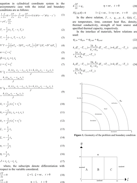
2. 1. Direct Problem The geometry of this problem is presented in Figure 1. As shown, a constant heat flux is applied in outer surface while the inner surface and side surfaces have been insulated. We aim to obtain the unknown strength of the heat source G(t) for the time

f t t£ £

0 _{in the outer layer using the temperature field at}

a point in the inner layer. The input data could include noise. In the numerical solution, the general coordinate method is applied. The calculations have been done in the rectangular coordinate system _{( )}x,h initially, and

then the results transfer to physical coordinate system (r − z). Thus, we used the chain rule of differential calculus. For solving the problem, the finite difference method in computational plane was used which in the grid space is uniform in

( )

x,h directions. The

equation in cylindrical coordinate system in the axisymmetric case with the initial and boundary conditions are as follows:

* *

1

( ) ( ) ( ) ( ) ( )

P

T T

k r k G t r r z z

r r r z z

T C t d d r ¶ ¶ ₊ ¶ ¶ _{+ -} -¶ ¶ ¶ ¶ ¶ = ¶ (1) ) ( 1 h x x hT r T

r J

Tz = - (2)

) ( 1 h x x hT z T

z J

Tr = - + (3)

2 2 2

2 1

2 ( ) ( )

T T T T T T

J éa xx b x h g hhù é x x h hù

Ñ = _ë - + _û+ Ñ_ë + Ñ _û (4)

2 2

h h

a=z +r (5)

h x h x

b=z z +r r (6)

2 2

x x

g =z +r (7)

J r z z r k J r z z r k r z z r k ) ( ) ( ) ( 3 2 1 2 h hh h hh h xh h xh h x x h xx x -+ -+ -= Ñ (8) J z r r z k J z r r z k z r r z k ) ( ) ( ) ( 3 2 1 2 x hh x hh x xh x xh x x x x xx h -+ -+ -= Ñ (9) ) (

1 2 2

2

1 _J zh rh

k = + (10)

) (

2

2

2 zxzh rxrh

J

k =- + (11)

) (

1 2 2

2

3 _J zx rx

k = + (12)

h x r J z 1 = (13) h x z J r 1 -= (14) x h r J z 1 -= (15) x h z J r 1 = (16) h x h

xr r z

z

J = - (17)

where, the subscripts denote differentiation with respect to the variable considered.

0

= ¶ ¶

z

T _{x=1, x=nz, t >0}

(18) 0 = ¶ ¶ r

T _{h =1, t >0}

(19) w q r T k = ¶

¶ _{h=nr, t >0}

(20)

(

x,h,0

)

=0

T 1< <x nz, 1< <h nr, t=0 (21) In the above relation, T, , t qw, , , G(t), r k Cp

are temperature, time, constant heat flux, density, thermal conductivity, strength of heat source and specified thermal capacity, respectively.

In the interface of materials, below relations are used:

out out in

in q q q

qx + h = x + h (22)

, 1, , 1, 1, ,

, 1 ,

2

( ) .( ) ( )

2 _{( )}

A B

A i j i j i j i j B i j i j

A B

A B

i j i j

A B

k k

k T T T T k T T

k k k k _{T T} k k - - + + - + + = -+ + + + (23)

, 1, , 1, 1, ,

, 1 ,

2

( ) .( ) ( )

2

( )

C B

B i j i j i j i j C i j i j

C B

C B

i j i j

C B

k k

k T T T T k T T

k k k k T T k k - - + + - + + = -+ + + + (24)

Figure 1. Geometry of the problem and boundary condition

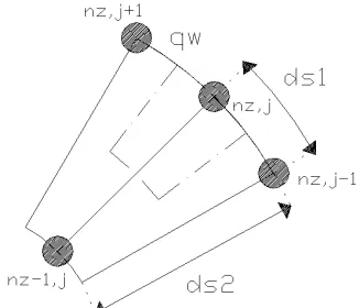
Figure 3. Boundary element in physical plane

As is shown in Figure 3, by considering a boundary element in physical plane and applying the energy equation, the boundary conditions are calculated as follows:

1 1 1 1

1, , 2 , 1 ,

, 1 ,

2 1

1 1

, 1 ,

2 , 1 1 1 , , 2

, , 1

2

2

( )

2

n n n n

nz j nz j nz j nz j

i j i j

n n

nz j nz j

i j w

n n

nz j nz j i j i j

T T ds T T

k ds k

ds ds

T T

ds

k q ds

ds T T ds C ds t r - - - -- -- -+ -- -+ + -+ = -D (25)

where, n j nz

T , in the above relation is as:

,

1 ,

, , 2

1 2

( 1 2 ( ) )

n n z j

n w

nz j

i j i j

T

q t

F T - A A _{r C ds}

=

D

+ + + (26)

, ,

2 2

1 , 2 ,

2 2

1 i j i j

n z j n z j

t t

F

d s d s

a D a D

= + + (27)

1

, 1 ,

1 2

2 ,

2 n

i j n z j

n z j t T A d s a -D = (28) 1 1

, , 1 , 1

2 2

1 ,

( n n )

i j nz j nz j

nz j

t T T

A

ds

a -

-+ -D + = (29) , , , i j i j i j k C

a = (30)

With similar method for other boundary conditions, we have: ) 2 1 ( 1 1 , 1 , 1 A A T F T _n j n j + +

= _{- (31)}

2 , 21 , 2 , 11 , 2 2 1 j j i j j i ds t ds t

F = + a D + a D (32)

2 , 21 1 , 2 , 1 2 j n j j i ds T t A -D

= a (33)

1 1

, 1, 1 1, 1

2 2

11,

( n n )

i j j j

j

t T T

A

ds

a -

-+ -D + = (34) , , , i j i j i j k C

a = (35)

,1 1

,1 1

( 1 2)

n

i n

i

T

F T - A A

=

+ + (36)

, ,

2 2

1 ,1 2 ,1

2 2

1 i j i j

i i

t t

F

ds ds

a D a D

= + + ₍₃₇₎

1

, ,2

1 2

1 ,1

2 n

i j i i

t T A

ds

a _D

-= (38)

1 1

, 1,1 1,1

2 2

2 ,1

( n n )

i j i i

i

t T T

A

ds

a -

-+ -D + = (39) , , , i j i j i j k C

a = ₍₄₀₎

2. 2. Inverse Problem In inverse problem, the strength of the time- dependent heat source using measured transient temperatures is estimated with a sensor positioned at a point. The inverse problem should be solved as the following function is minimized:

( )

[Gt ] [T( t G) Y ( )t ]dt S

f

t

t NS

m m m m

ò å

= = -= 0 1 2 ; , , 2

1 _{x h (41)}

In the above relation, T

(

x_m,h_m,t;G

)

, Y_m

( )

t are estimated temperatures and measured temperature, respectively. Also, number of sensors Ns is equal to 1.

The above equation will be minimized using the conjugate gradient method based on iterative processes. In the conjugate algorithm, the direction of seeking the unknown heat source is depend on the gradient of the error function which will be solved with adjoint equation [10, 11, 15]:

2. 2. 1. Adjoint Problem

( ) ( ) ( ) ( ) 1 , , ; 1 ( ) ( ) NS

m m m

m

P

T t q Y t

k r k C

r r r z z t

x h d h h d x x

l l l

r = - - -é ù ë û ¶ ¶ ¶ ¶ ¶ + + = ¶ ¶ ¶ ¶ ¶

å

(42) 0 = ¶ ¶ z

l _{x=1, x =nz, t >0}

(43) 0 = ¶ ¶ r

l _{h=1, h=nz, t >0}

(44)

(

x,h,tf

)

=0

l 1< <x nz, 1< <h nr t, =tf (45)

In the interface of materials, below relations are used:

, 1, , 1, 1, ,

, 1 ,

2

( ) ( ) ( )

2

( )

A B

A i j i j i j i j B i j i j

A B

A B

i j i j

A B k k k k k k k k k k

l l l l l l

, 1, , 1, 1, ,

, 1 ,

2

( ) ( ) ( )

2

( )

C B

B i j i j i j i j C i j i j

C B

C B

i j i j

C B k k k k k k k k k k

l l l l l l

l l - - + + - + + = -+ + + + (47)

where, the l parameter is adjoint temperature and

d

is dirac delta function.

The optimum step size can be obtained based on the sensitivity problem which is defined as in some references [11, 15].

2. 2. 2. Sensitivity Problem To obtain the sensitivity equation, it is assumed that perturbing G

( )

t

by DG(t) would change T(r,z,t) by DT(r,z,t). Thus, in direct problem the quantities T(r,z,t) and G

( )

t are

replaced by

[

T(r,z,t)+DT(r,z,t)

]

and

[

G(t)+DG(t)

]

;then,

the resulting expression is subtracted from the direct problem. In this way, the sensitivity equation is obtained as: * * 1 ( ) ( ) ( ) ( ) ( ) p T T

k r k G t r r z z

r r r z z

T c

t

d d

r

¶ ¶D ₊ ¶ ¶D _{+ D -}

-¶ ¶ ¶ ¶ ¶ D = ¶ (48) 0 = ¶ D ¶ z

T _{x =1, x =nz, t >0}

(49) 0 = ¶ D ¶ r

T _{h=1, t>0}

(50) 0 = ¶ D ¶ r

T _{h =nr, t >0}

(51)

(

, ,0

)

=0

DTxh 1< <x nz, 1< <h nr, t=0 (52) In the interface of materials, below relations are used:

, 1, , 1,

1, , , 1 ,

2

( ) ( )

2

( ) ( )

A B

A i j i j i j i j

A B

A B

B i j i j i j i j

A B

k k

k T T T T

k k k k

k T T T T

k k

-

-+ +

D - D + D + D

+

= D - D + D + D

+

(53)

, 1, , 1,

1, , , 1 ,

2

( ) ( )

2

( ) ( )

C B

B i j i j i j i j

C B

C B

C i j i j i j i j

C B

k k

k T T T T

k k

k k

k T T T T

k k

-

-+ +

D - D + D + D = +

D - D + D + D +

(54)

where, DT is the sensitivity temperature.

The transient heat source G

( )

t which is an unknown function can be estimated by minimizing the function

[

G(t)

]

S in the Equation (41).The iterative equation for estimating the G

( )

t is as below [10, 12, 15]:

( ) ( ) ( )

1 _Gk _- k_dk

k

G + t ₌ t b t

(55) In which k is the number of iteration. The direction of descent dk

( )

t _{is determined [10, 12, 15]:}

( ) _{S G}k( ) k_dk-1( )

k

d t = Ñ é_ë t ù_û+g t (56)

Here, _gk _{is the conjugate coefficient [11, 13, 15] which} is calculated by:

{

[

]

}

[

]

{

}

ò

ò

= -= Ñ Ñ = f f t t k t t k k dt t G S dt t G S 0 2 1 0 2 ) ( ) ( g (57)

where, _g0 _{is assumed zero. To calculate ÑS}

[

_Gk

( )

_t

]

_{, the}

following relation is used:

( )

[

G t

]

( , ,t)

S k _{=l x h}

Ñ (58)

The above equality depends on the position of unknown function. The search step-size, _bk _{is obtained}

by minimizing S

[

Gk+1

( )

t

]

_{with respect to b}k _{as follows} [11, 13, 15]:

(

)

( )

(

)

(

)

1 0 2 1 0 , , ; . , , ; , , ; f f t NS k k

m m S m m

m k t t _NS k m m m t

T t G Y t T t d dt

T t d dt

x h x h

b x h = = = =

é - ùD

ë û

=

éD ù

ë û

å

ò

å

ò

(59)

where,

(

k

)

m

m td

Tx ,h , ;

D is obtained from sensitivity

problem by considering _DGk

( )

t ₌dk

( )

t _.

By checking the Equation (58), it is determined that the gradient equation in final time ( )tf is equal to zero.

Therefore, the initial guess used for G_{( )}t in t=t_f

doesn’t change with iterative process in conjugate gradient method. When the initial guess is very far from exact solution, the estimated function in the neighborhood of t_f can deviate from the exact solution. This solution can be eliminated easily by use of a larger value of final time. Thus, the effect of initial guess on the actual time of the problem is not significant. The iterative procedure mentioned above, continues until the stopping criterion is satisfied. The stopping criterion is defined as follows:

( )

[ ]

Gt £e

S (60)

In the above relation, S

[

G(t)

]

is obtained from Equation (41). The value of

e

should be selected such that, if there were errors in the measured data, the accuracy of the results would be satisfactory.

2. 2. 3. Computational Algorithm The computational procedure for obtaining the unknown heat source can be summarized as follows:

1- Choose an initial guess for example _G0(_t) _{for the} function G(t)and set k=0.

2- Solve the direct problem to obtain T

(

z,r,t

)

based on

) (t

Gk (Equations (1-24)).

4- Solve the adjoint equation and compute the

(

x,nr,t

)

l by knowing T

(

x_m,h_m,t

)

and the measured temperature Y_m

( )

t ( Equations (42-47)).

5- Knowing l

(

x,nr,t

)

, compute _ÑS

[

Gk

( )

t

]

_from

Equation (58).

6- Knowing _ÑS

[

Gk

( )

t

]

_{, compute g}k _{from Equation (57)}

and dk(t)_{from Equation (56).}

7- Set _DGk

( )

t ₌dk(t) _{and solve the sensitivity problem}

to obtain

(

k

)

m

m td

Tx ,h , ;

D (Equations (48-54)).

8- Knowing

(

k

)

m

m t d

Tx ,h , ;

D , Compute _bk _from

Equation (59).

9- Knowing _bk _{and d}k_{(t), compute G}k+1

( )

_{t and return}

to step 2, (Equation (55)).

3-RESULTS AND DISCUSSIONS

We aim to estimate the unknown strength of heat source using conjugate gradient method when there is no information about unknown function. It should be noted that in conjugated gradient method the initial guess for unknown function is arbitrary. In other word, the method is independent of initial guess. Here, initial estimation for heat source is assumed zero. The governing equations were discretized by the finite-difference method and the mesh size used in numerical is a uniform 35x35. The final time t_f =10 and time step

01 . 0 =

Dt are considered. In this work, by measuring the temperature at a point only, the heat source is estimated and the sensitivity of the problem for a noisy data is investigated. In Figure 4, the mesh used and the position of sensors is shown.

The temperature data obtained from the direct problem are used to simulate the temperature measurement.

Figure 4. using grid in solution of problem and sensor

position

To investigate the accuracy of the presented solution, a step function is considered as:

( ) î í ì

³ £

< < =

8 4 0

8 4 107

t and t for

t for t

G

One should note that the discontinuous and sharp corner functions are well known for being highly ill-posed. Therefore, these functions can be used to evaluate the accuracy of the solutions.

In the next example, as it shown in Figure 6, a sinusoidal function is considered for the heat source as:G

( )

t ₌107sin

( )

pt _{. In the other example which is}

shown in Figure 7, a combination of sine and cosine functions is considered for the heat source as:G

( )

t ₌107sin

(

0.1t

)

₊107cos

( )

2t .

Figure 5. Estimated heat source in comparison with exact

function for Step-function

Figure 6. Estimated heat source in comparison with

Figure 7. Estimated heat source in comparison withexact function for a combination of sine and cosine functions

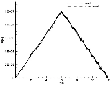
In the next example, a triangle function is considered for the heat source.

Figure 8. Estimated heat source in comparison with exact

function for triangle function

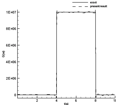
Figure 9. Estimated heat source with noisy data in comparison

with Exact-function for step-function

Figure 10. Estimated heat source with noisy data in

comparison with exact function for sine function

Figure 11. Estimated heat source with noisy data in

comparison with exact function

In this part, the inverse solution with noisy data is presented. In practice, there are errors in measured data; therefore noisy data are used to simulate the errors and using a data with 4% noise. The effect of noisy data can be seen in Figures 9-12 in comparison to noiseless cases (Figures 5- 8). It is found that despite a noise in data, results have very good stability.

Figure 12. Estimated heat source with noisy data in

4. CONCLUSIONS

The conjugate gradient method with adjoint problem has been successfully applied for the solution of inverse heat conduction to estimate the unknown time-depended heat source using the temperature distribution at a point in a three layer system. The general coordinate method is also used. Since, in the most of industrial applications, axisymmetric models are used, for example: in thermal protect systems (t.p.s) and heat shield systems, we use an axisymmetric model. The present formulation is general and can be applied to the solution of inverse heat conduction problems over any region that can be mapped into a rectangle. In this paper, the discontinuous and sharp corner functions that are well known for being highly ill-posed were used for illustrating the good accuracy of presented method. The obtained results show that the presented solution has good stability even when there is a noise in input data up to 4%. Therefore, the presented method is a good method for estimating the time-dependent unknown heat source in multi layer systems.

5. REFERENCES

1. Huang, C.H. and Wang, P., "A three-dimensional inverse heat conduction problem in estimating surface heat flux by conjugate gradient method", International Journal of Heat and Mass Transfer, (1999), 3387-3403.

2. Shiguemori, E.H., Harter, F.P., Campos Velho, H.F., and da Silva, J.D.S., "Estimation of boundary conditions in conduction heat transfer by neural networks", Tendˆencias em Matem´atica Aplicada e Computacional, Vol. 3, No. 2, (2002), 189-195.

3. Volle, F., Maillet, D., Gradeck, M., Kouachi, A., and Lebouché, M., "Practical application of inverse heat conduction for wall condition estimation on a rotating cylinder", International Journal of Heat and Mass Transfer, Vol. 52, (2009), 210–221.

4. Golbahar Haghighi, M.R., Eghtesad, M., Malekzadeh, P. and Necsulescu, D.S., "Three-dimensional inverse transient heat transfer analysis of thick functionally graded plates", Energy Conversion and Management, Vol. 50, (2009), 450–457.

5. Su, J. and Neto, A., "Two dimensional inverse heat conduction problem of source strength estimation in cylindrical rods",

Applied Mathematical Modeling, Vol. 25, (2001), 861- 872.

6. Hsu, P.T., "Estimating the boundary condition in a 3D inverse hyperbolic heat conduction problem", Applied Mathematics and Computation, Vol. 177, (2006), 453–464.

7. Shi, J. and Wang, J., "Inverse problem of estimating space and time dependent hot surface heat flux in transient transpiration cooling process", International Journal of Thermal Sciences, Vol. 48, (2009), 1398–1404.

8. Ling, X. and Atluri1, S.N.,"Stability analysis for inverse heat conduction problems", Tech Science Press, CMES, Vol. 13, No.3, (2006), 219-228.

9. Jiang, B.H., Nguyen, T.H. and Prud’homme, M., "Control of the boundary heat flux during the heating process of a solid

material", International Communications in Heat and Mass Transfer, Vol. 32, (2005), 728–738.

10. Jarny, Y., Ozisik, M.N. and Bardon, J.P., "A General Optimization Method Using Adjoint Equation for Solving Multidimensional Inverse Heat Conduction", Journal of Heat and Mass Transfer, Vol. 34, (1991), 2911-2919.

11. Daniel, J.W., "Approximate Minimization of Functionals", Prentice-Hall Inc. Englewood Cliffs, (1971).

12. Ozisik, M.N., "Heat Conduction", 2nd _{ed., Wiley, New York,}

(1993).

13. Alifanov, O.M., "Inverse Heat Transfer Problems", Springer-Verlag, New York, (1994).

14. Chen, S.G., Weng, C.I. and Lin, J., "Inverse estimation of transient temperature distribution in the end quenching test",

Journal of Materials Processing Technology, Vol. 86, (1999), 257–263.

15. Ozisik, M.N. and Orlando, R.B., "Inverse Heat Transfer", New York, Taylor & Francis, (2000).

16. Chen, C.K., Wu, L.W. and Yang,Y.T., "Application of the inverse method to the estimation of heat flux and temperature on the external surface in laminar pipe flow", Applied Thermal Engineering, Vol. 26, (2006), 1714-1724.

17. Lagier, G.L., Lemonnier, H. and Coutris, N., "A numerical solution of the linear multidimensional unsteady inverse heat conduction problem with the boundary element method and the singular value decomposition", International Journal of Thermal Sciences, Vol. 43, (2004), 145-155.

18. Yang, Y.C., Chu, S.S., Chang, W.J. and Wu, T.S., "Estimation

of heat flux and temperature distributions in a composite strip

and homogeneous foundation", International Communications

in Heat and Mass Transfer, Vol. 37, (2010), 495–500.

19. Bao Liu, F., "A hybrid method for the inverse heat transfer of estimating fluid thermal conductivity and heat capacity",

International Journal of Thermal Sciences, Vol. 50, (2011), 718-724.

20. Chen, T.C., Liu, C.C., Jang, H.Y. and Tuan, P.C., "Inverse estimation of heat flux and temperature in multi-layer gun barrel", International Journal of Heat and Mass Transfer, Vol. 50, (2007), 2060–2068.

21. Gutiérrez Cabeza, J.M., Martín García, J.A. and Corz Rodríguez, A., "A sequential algorithm of inverse heat conduction problems using singular value decomposition", International Journal of Thermal Sciences, Vol. 44, (2005), 235-244.

22. Gejadze, I. and Jarny, Y., "An inverse heat transfer problem for restoring the temperature field in a polymer melts flow through a narrow channel", International Journal of Thermal Sciences, Vol. 41, (2002), 528-535.

23. Kakaee, A.H. and Farhanieh, B., "Development of a moving finite element based inverse heat conduction method for determination of moving surface temperature", International journal of engineering, Transaction A, Vol. 17, No. 3, (2004), 281-292.

24. Mohammadiun, M. and Rahimi, A.B., "Estimation of the time- dependent heat flux using the temperature distribution at a point in a two layer system", Scientia Iranica, Transaction B, Vol. 18, No. 4, (2011), 966-973.

Estimation of the Strength of the Time-dependent Heat Source Using Temperature

Distribution at a Point in a Three Layer System

A. B. Rahimia _{, M. Mohammadiun}b

a _{Faculty of Engineering, Ferdowsi University of Mashhad, P.O. Box No. 91775-1111, Mashhad, Iran} b _{Department of Mechanical Engineering, Shahrood branch, Islamic Azad University, Shahrood, Iran}

P A P E R I N F O

Paper history: Received 7 January 2012

Received in revised form 1 July 2012 Accepted 30 August 2012

Keywords:

Time- dependent Heat Source Inverse Heat Conduction Problem General Coordinate

Three Layer System

هﺪﯿﮑﭼ

وﯽﺗراﺮﺣﺖﯾاﺪﻫسﻮﮑﻌﻣﻪﻟﺎﺴﻣﻞﺣﺎﺗدﻮﺷﯽﻣﻪﺘﻓﺮﮔرﺎﮐﻪﺑﯽﻗﺎﺤﻟاﻪﻟﺎﺴﻣﺎﺑهاﺮﻤﻫجودﺰﻣنﺎﯾداﺮﮔشورﻪﻟﺎﻘﻣﻦﯾارد دﻪﻄﻘﻧﮏﯾردتراﺮﺣﻪﺟردﻊﯾزﻮﺗزاهدﺎﻔﺘﺳاﺎﺑنﺎﻣزﻊﺑﺎﺗﯽﺗراﺮﺣﻊﺒﻨﻣتﻮﻗﻦﯿﻤﺨﺗ ﮏﯾر

ﺪﯾآﺖﺳدﻪﺑﻪﯾﻻﻪﺳﻢﺘﺴﯿﺳ

.

دﺮﯿﮔﯽﻣراﺮﻗﯽﺳرﺮﺑدرﻮﻣﯽﺋﺎﻬﻧﻞﺣردﯽﺘﯾزارﺎﭘيﺎﻫهدادﺮﺛاﻦﯿﻨﭽﻤﻫ

.

يﺮﯿﮔرﺎﮐﻪﺑﺎﺑﻢﮐﺎﺣتﻻدﺎﻌﻣيدﺪﻋﻞﺣ شور

ﺪﯾآﯽﻣﺖﺳدﻪﺑدوﺪﺤﻣﻞﺿﺎﻔﺗ

.

دﻮﺷﯽﻣهدﺎﻔﺘﺳاﯽﻣﻮﻤﻋتﺎﺼﺘﺨﻣهﺎﮕﺘﺳدشورزاﻪﻟﺎﺴﻣﻦﯾاﻞﺣياﺮﺑ

.

ﺖﯾاﺪﻫﻪﻟﺎﺴﻣ

ﻣتﻮﻗﻦﯿﻤﺨﺗسﻮﮑﻌﻣﯽﺗراﺮﺣ دﻮﺷﯽﻣﻪﺘﻓﺮﮔﺮﻈﻧردﻢﻈﻨﻣﺮﯿﻏﻪﯿﺣﺎﻧﮏﯾﻞﺧادردارﺬﮔﯽﺗراﺮﺣﻊﺒﻨ

.

ﻢﻈﻨﻣﺮﯿﻏﻪﯿﺣﺎﻧﻦﯾا

دﻮﺷﯽﻣهدادﻞﯾﺪﺒﺗﯽﺗﺎﺒﺳﺎﺤﻣهدوﺪﺤﻣردﯽﻠﯿﻄﺘﺴﻣﻞﮑﺷﮏﯾﻪﺑﯽﮑﯾﺰﯿﻓهدوﺪﺤﻣرد

.

ﯽﻣﻮﻤﻋترﻮﺻﻪﺑندﺮﮐﻪﻟﻮﻣﺮﻓﻦﯾا

راﺮﻗهدﺎﻔﺘﺳادرﻮﻣﻞﯿﻄﺘﺴﻣﮏﯾﻪﺑﻞﯾﺪﺒﺗﻞﺑﺎﻗهدوﺪﺤﻣﺮﻫردﯽﺗراﺮﺣﺖﯾاﺪﻫسﻮﮑﻌﻣﻞﯾﺎﺴﻣﻞﺣياﺮﺑﺪﻧاﻮﺗﯽﻣوهدﻮﺑ دﺮﯿﮔ

.

ياﺮﺑهﺪﻣآﺖﺳدﻪﺑﺞﯾﺎﺘﻧ ﺪﺷﺎﺑﯽﻣهدﺎﻔﺘﺳادرﻮﻣشورزابﻮﺧﺖﻗدهﺪﻨﻫدنﺎﺸﻧﯽﺑﺎﺨﺘﻧالﺎﺜﻣﺪﻨﭼ

.

ﯽﺘﺣﺞﯾﺎﺘﻧﻦﯾا

ﺪﺷﺎﺑﯽﻣﯽﺑﻮﺧيراﺪﯾﺎﭘيارادﺰﯿﻧﺖﯾزارﺎﭘﻞﻣﺎﺷيﺎﻫهدادياﺮﺑ

.