Point-wise integrated-RBF-based discretisation of differential equations

(1)

Point-wise Integrated-RBF-based Discretisation of

Differential Equations

Nam MAI-DUY

a,

*

and Thanh TRAN-CONG

a

a_{Computational Engineering and Science Research Centre}

Faculty of Engineering and Surveying

University of Southern Queensland, Toowoomba, QLD 4350, Australia (*[email protected])

Abstract. This paper discusses a discretisation scheme which is based on point collocation and integrated radial basis function networks (IRBFNs) for the solution of elliptic differential equations (DEs). The use of IRBFNs to represent the field variable in a given DE gives several advantages over the case of using conventional RBFNs and polynomials. Some numerical examples are included for demonstration purposes.

Keywords: Integrated RBFs, Point collocation, PDEs.

PACS: 02.70.Jn, 02.70.Hm, 87.10.Ed

INTRODUCTION

Computational methods for DEs can be classified into two groups: low- and high-order discretisation schemes. The former (e.g. conventional finite-difference, finite-element and finite-volume methods) produces a system of algebraic equations which is sparse and can be solved efficiently. However, very dense meshes are typically required to achieve accurate results. The latter (e.g. spectral methods) has the ability to give a high level of accuracy using a relatively-coarse mesh. However, the structure of its system matrices is typically full.

RBFNs are a high-order interpolation scheme (e.g. [1]). Unlike schemes based on Chebyshev polynomials and Fourier series, RBFNs do not require an underlying structured discretisation. Some RBFs such as Gaussian and multiquadric functions can offer an exponential rate of convergence. Theoretical results indicated that the convergence order of an RBFN scheme is a decreasing function of derivative order.

Point collocation is regarded as the simplest means of discretising an DE, where no integrations are required. One disadvantage of the point-collocation approach is that it is seen, in general, not to be as stable as the weak-form approach.

In this paper, we discuss a computational procedure, based on RBFNs and point collocation, for solving elliptic problems. A distinguishing feature here is that the RBFN approximations are constructed through integration (IRBFNs) rather than conventional differentiation (DRBFNs). This use of integration helps to avoid the problem of reduced convergence rate in the approximation of derivative functions. Furthermore, the constants of integration can be utilised as extra coefficients from which one can straightforwardly incorporate extra information such as the DE on the boundaries and derivative boundary values into the discrete system. The discussion is based on some of our previous works on IRBFNs reported in [2-6]. For simplicity, our attention is limited to the case of one-dimensional problems.

(2)

REVIEW OF IRBFNs

Consider a univariate function

u(x)

. The integral formulation [2,3] tries to decompose the highest-order derivatives of

u

under consideration, e.g.

p

, into RBFs and then integrate them to obtain approximate expressions for lower-order derivatives and the function itself

(

)

(

)

p p

p p n i i i n i p i i p p n i p i i n i i i p p

c

x

c

p

x

c

p

x

c

x

I

u

c

x

I

dx

x

u

d

x

I

x

dx

x

u

d

+

−

+

−

+

=

+

=

− − − = = − − − = =

∑

1 2 2 1 1 1 ) 0 ( 1 1 ) 1 ( 1 1 1 ) ( 1

!

2

!

1

)

(

)

(

)

(

)

(

)

(

)

(

L

K

α

ϕ

α

(1)

where

{ }

α

_i _in₌₁ is the set of expansion coefficients;

{

ϕ

_i

(

x

)

}

_in₌₁

=

{

I

_i(p)

(

x

)

}

_in₌₁ the set of RBFs;

{ }

c

_i _ip₌₁ the set of integration constants; and

I

x

I

x

dx

I

i

x

I

i

x

dx

p i p

i

=

∫

=

∫

−

)

(

)

(

,

)

(

)

(

( ) (0) (1)

) 1

(

L

. The integral approximation scheme is said to be of order p, denoted by IRBFN-p, if the pth-order derivative is taken as the starting point. Collocation a function

u

and its derivatives at a set of collocation points

{ }

n

j j

x

1

= leads to

s

u

s

dx

u

d

s

dx

u

d

p p p p p p p p p

r

L

r

) 0 ( ] [ ) 1 ( ] [ 1 1 ) ( ] [

ℑ

=

ℑ

=

ℑ

=

− − − (2)

where the subscript [.] and superscript (.) are used to indicate the order of the IRBFN scheme and the order of the corresponding derivative function, respectively;

(

)

T

p n

c

s

r

=

α

₁

,

α

₂

,

L

,

α

,

₁

,

₂

,

L

,

(3)

( )













−

=

ℑ

− − − − − −

1

)!

2

(

)!

1

(

)!

2

(

)!

1

(

)!

2

(

)!

1

(

2 1 2 2 2 1 2 1 2 1 1 1 ) 0 ( ) 0 ( 2 ) 0 ( 1 2 ) 0 ( 2 ) 0 ( 2 2 ) 0 ( 1 1 ) 0 ( 1 ) 0 ( 2 1 ) 0 ( 1 ) 0 ( ] [

M

L

M

O

M

L

M

O

M

L

n p n p n p p p p n n n n n n p

x

p

x

p

x

p

x

p

x

p

x

p

x

I

x

I

x

I

x

I

x

I

x

I

x

I

x

I

x

I

(6)

{

}

(

)

T

n T k n k k k k k k k

u

p

k

dx

u

d

dx

u

d

dx

u

d

dx

u

d

,

2

,

1

,

2 ₁ ₂

1

L

=

L

r

=

L













=

(7)

in which j k

k k j k

dx

x

u

d

dx

u

d

=

(

)

and

u

j

=

u

( )

x

j with

j

=

{

1

,

2

,

L

,

n

}

.

POINT-WISE IRBFN TECHNIQUE

In the remainder of the paper, we will use the notation

[]

(η,θ)to denote selected rows

η

and columns

θ

of the matrix [],

[]

₍_η₎ to pick out selected components

η

of the vector [],

[]

_(:,_θ₎ to denote all rows of the matrix [], and

,:) (

[]

_η to denote all columns of the matrix [].

Consider a boundary-value problem governed by the pth-order DE

s

x

r

x

b

dx

u

d

dx

u

d

dx

du

u

F

_p p

≤

=













),

(

,

₂ 2

L

₍₈₎

where F and b are prescribed functions, with boundary conditions for u, du/dx, ...,

d

p/2−1

u

/

dx

p/2−1 at x=r and

x=s.

The continuous domain of interest is represented by a set of discrete points

{ }

n

j j

x

1

= with

x

1

=

r

and

x

n

=

s

. The

integral scheme of order p (IRBFN-p) is employed here to approximate the field variable

u

. Owing to the presence of

p integration constants, one can add p extra equations to the discrete system. These extra equations can be utilised to represent the DE and the values of the derivative boundary conditions at both ends of the domain. The governing equation and the boundary conditions can be transformed into the following discrete form

f

r

=

ℜ

α

(9) where

ℜ

is the system matrix of size

(

n

+

p

) (

×

n

+

p

)

defined as

(4)

(

)

T p n

,

c

,

c

,

c

,

₂ ₁ ₂

1

L

r

α

=

(11)













=

₋

−

− −

1 2 /

2

1

,

p

s p p

r p s

r s r n

dx

u

d

dx

u

d

dx

du

dx

du

u

b

f

L

r

(12)

It can be seen that the DE is collocated at all grid points including the two boundary points x=r and x=s.

NUMERICAL RESULTS

We will implement IRBFNs with the multiquadric (MQ) function (

ϕ

i

(

x

)

=

(

x

−

x

i

)

2

+

a

i2

,

x

i and

a

i–the

centre and the width). The two sets of centres and collocation points are chosen to be identical and the MQ width is taken as the centre spacing. We measure accuracy of an approximate scheme through the relative

L

₂ norm denoted by

N

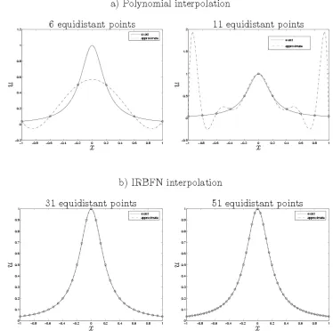
e. [image:4.595.106.480.328.700.2]

Runge’s Phenomenon

(5)

When using algebraic polynomials to represent certain functions that are sampled at equally-spaced points, the error between the function and the interpolating polynomial can grow quickly as the number of sample points increases, which is called Runge's phenomenon. Figure 1a illustrates this phenomenon for the interpolation of a function

u

(

x

)

=

1

/(

1

+

25

x

2

),

−

1

≤

x

≤

1

. The oscillation between the interpolating points, especially in the region close to the boundaries, is significantly magnified when changing from 6 to 11 points. To minimise/eliminate the oscillation, it is necessary to employ Chebyshev nodes that cluster at the boundaries of the domain or to use piecewise low-order polynomials. For the latter, the quality of the interpolation is improved by increasing number of polynomial pieces. [image:5.595.156.420.249.455.2]

It is interesting to see the behaviour of IRBFNs when they are applied to interpolate the above function. As shown in Figure 1b, there is no oscillation between the interpolating points for the IRBFN-2 scheme. Indeed, the interpolation error is reduced with increasing number of equidistant points. IRBFNs can thus work well with the equidistant points.

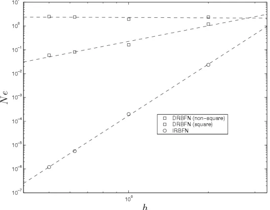
FIGURE 2. High-order DE: accuracy by DRBFNs and IRBFNs

Multiple Boundary Conditions

The problem here is to find a function

u(x)

satisfying the following fourth order DE

(

)

₂

(

2

)

(

2

)

5

2 2 2

3 3 3 4 4 4

2

12

2

12

2

12

4

x

u

x

dx

du

x

dx

u

d

x

dx

u

d

x

dx

u

d

x

−

+

−

+

−

+

−

=

(13) over a specified interval

1

≤

x

≤

11

, subject to the boundary conditions for

u

and

du/dx

at both ends of the

domain. The exact solution can be verified to be

u

x

=

x

+

x

2

−

x

3

+

xe

x

+

xe

−x

)

(

. To study convergence, four sets of 6, 11, 17 and 21 equally-spaced points are employed for both DRBFNs and IRBFN-4s. For all study cases,

e

N

s of the solution u are calculated at a test set of 101 uniformly-distributed points. By collocating the DE at the whole set of grid points, the integral and differential approaches produce square and non-square (over-determinated) systems, respectively. For the latter, by not applying the DE at two boundary points together with two interior points (for example, interior points adjacent to the boundaries are set aside here), the system becomes determinated. Figure 2 shows that the integral approach yields very accurate results and also a high convergence rate while the opposite is true for the conventional differential approach. Solutions converge apparently as

O

(

h

−0.04

)

,

O

(

h

2.17

)

and

(

7.16

)

h

(6)

Higher-Order Smoothness of the Solution Across the Subdomain Interfaces

Consider the following second-order DE

5

[

9979

sin(

100

)

900

cos(

100

)

]

,

0

1

2 2

≤

+

−

=

+

u

e

−

x

dx

du

dx

u

d

x

(14)

with Dirichlet boundary conditions

u

(0)=0

and

u

(

1

)

=

sin(

100

)

e

−5. The exact solution can be verified to be

x

e

x

u

(

)

=

sin(

100

)

−5 which is highly oscillatory. The domain is partitioned into two subdomains of the same size, and each subdomain is discretised with uniformly-distributed points. Ten grids are considered with their densities varying from 21 to 201 in increment of 20. A test set of 201 uniform points is used to compute the error

e

N

.

Unlike DRBFNs, IRBFN-2s allow the exact satisfaction of the DE at the interface points. As a result, the approximate solution is a

C

1 function across the interface for DRBFNs and

C

2 for IRBFNs. Table 1 presents

N

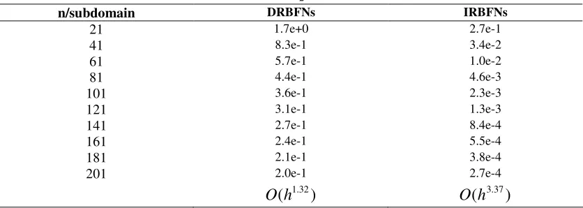
es [image:6.595.89.507.322.471.2]

of DRBFNs and IRBFNs. The performance of the latter is far superior to that of the former regarding both accuracy and convergence rate.

TABLE 1. Domain decomposition, 2 subdomains:

L

₂ errors by the differential and integral approaches.

n/subdomain DRBFNs IRBFNs

21 1.7e+0 2.7e-1

41 8.3e-1 3.4e-2

61 5.7e-1 1.0e-2

81 4.4e-1 4.6e-3

101 3.6e-1 2.3e-3

121 3.1e-1 1.3e-3

141 2.7e-1 8.4e-4

161 2.4e-1 5.5e-4

181 2.1e-1 3.8e-4

201 2.0e-1 2.7e-4

)

(

h

1.32

O

(

h

3.37

)

CONCLUSIONS

In this paper, we discuss the use of IRBFNs in the point-collocation scheme for solving elliptic DEs. The employment of integration to construct the RBF approximations has the capability to enhance the quality of the approximation of derivative functions. Further attractive features include: (a) uniformly-distributed points can be employed for the discretisation without suffering from Runge’s phenomenon, (b) extra information can be incorporated into the discrete system in a proper way, and (c) the approximate solution achieves a higher order of smoothness across the subdomain interfaces. Results obtained from various test problems are very encouraging.

ACKNOWLEDGMENTS

This work is supported by the Australian Research Council

REFERENCES

1. G. E. Fasshauer, Meshfree Approximation Methods With Matlab, Singapore: World Scientific Publishers, 2007. 2. N. Mai-Duy and T. Tran-Cong, Applied Mathematical Modelling, 27, 197—220 (2003).

3. N. Mai-Duy and T. Tran-Cong T, Neural Networks, 14, 185—199 (2001).

4. N. Mai-Duy, D. Ho-Minh D and T. Tran-Cong, International Journal of Computer Mathematics (accepted, 24-Nov-2008). 5. N. Mai-Duy and T. Tran-Cong, Numerical Methods for Partial Differential Equations, 24, 1301—1320 (2008).