Abstract-The Newton-Raphson method is one of the most
widely used methods for minimization. It can be easily generalized for solving non-linear differential equation systems. In this study, Generalized Predictive Controller (GPC) was applied to a 6R robot manipulator based on joint control. Newton-Raphson (N-R) method was used to minimize the cost function existing in the GPC that represents errors between reference trajectory and actual trajectory in the control of robot. The Newton-Raphson method requires less iteration numbers for convergence and reduces the calculation. This study presents a detailed derivation of the Generalized Predictive Control algorithm with Newton-Raphson minimization method. The results of angular path and position errors belonging to joints were examined and compared with Recursive Least Square (RLS) implemented Generalized Predictive Control. The simulation results showed that Newton-Raphson method improved control performance of the GPC.
Keywords- Predictive control, generalized predictive control,
cost function minimization.
I. INTRODUCTION
Predictive control algorithm was developed from the non-parameter model predictive control algorithm including the Model Algorithm Control (MAC), the Dynamic Matrix Control (DMC) and so on, to the Model Predictive Control (MPC) algorithm on example of which is the Generalized Predictive Control (GPC) algorithm [1-4]. Because the GPC algorithm parameter model is shorter than the non-parameter model, it reduced the GPC algorithm calculation time, and enhanced performance of the control system.
The GPC is used in the control of non-minimum phase plants, open-loop unstable plants and plants with variable or unknown dead time. It is also robust with respect to modeling errors, over and under parameterization, and sensor noise [5-6].
The computational performance of a GPC implementationis
Manuscript received November 3, 2007. This work was supported by scientific research fund (University of Sakarya, grant no. 2006.50.02.050).
B.Durmuş is with Sakarya University, Department of Electric - Electronic Engineering, 54187 Adapazari, TURKEY (corresponding author phone: +90-533-5494170; fax: +90-264-2955601; e-mail: bdurmus@ sakarya.edu.tr).
H. Temurtaş Dumlupınar University, Department of Electric - Electronic Engineering, 41470 Kutahya, TURKEY (e-mail: [email protected]).
N. Yumuşak Sakarya University, Department of Computer Engineering, 54187 Adapazari, TURKEY (e-mail: [email protected]).
F. Temurtaş Sakarya University, Department of Computer Engineering, 54187 Adapazari, TURKEY (e-mail: [email protected]).
R. Kazan Sakarya University, Department of Mechanical Engineering, 54187 Adapazari, TURKEY (e-mail: [email protected]).
largely based on the minimization algorithm chosen for its CFM block. There are several minimization algorithms that have been implemented in GPC such as Non-gradient [7], Simplex, and Successive Quadratic Programming [8,9]. The selection of a minimization method can be based on several criteria such as; number of iterations to a solution, computational costs and accuracy of the solution. In general these approaches are iteration intensive thus making real-time control difficult. Very few papers address real-real-time implementation or the they used plants with large time constant [8,9]. To improve the usability, a faster optimization algorithm is needed. The Newton-Raphson method is one of the most widely used methods for minimization. It is a quadratic algorithm converging better than others. It requires less iteration numbers for convergence and reduces the calculation.
In this study, Generalized Predictive Control (GPC) was applied to 6R robot manipulator for joint control. Newton-Raphson (N-R) method was used to minimize the cost function existing in GPC that represents errors between reference trajectory and actual trajectory in the control of robot. The results of angular path and angular velocity belonging to joints were examined and compared with results obtained from the Recursive Least Square implemented Generalized Predictive Control. Also, processing times of both algorithms were shown.
II. GENERALIZED PREDICTIVE CONTROL The Generalized Predictive Control (GPC) introduced by Clarke is a generalization of the model-based control and suitable for controlling of the processes with variable dead time and a plant which is simultaneously non-minimum-phase and open loop unstable. Many research showed the effectiveness of this control algorithm [3].
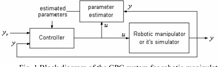
[image:1.595.314.535.679.747.2]The GPC system for the robotic manipulator is given in Figure 1. It consists of three components, the robotic manipulator or its simulator, controller and parameter estimator. Where, torque, u, is the control input to the manipulator system, the trajectory, y, is the output, and yr is the reference output.
Fig. 1 Block diagram of the GPC system for robotic manipulator
The heart of a model-based predictive controller is the plant model. The Controlled Autoregressive Integrated
The Cost Function Minimization for Predictive
Control by Newton-Raphson Method
Moving Average (CARIMA) model is commonly used in the GPC, as it is applicable to many input single-output plants:
∆ +
−
= −
− ) () ( ) ( 1) ( )/
(q 1 y t B q 1 ut t
A ξ (1)
Where, u(t), y(t) are the plant input and output. A and B are polynomials in the backward shift operator q-1:
∑
= − − = Ι + na
j j j m a q
q A
1 1)
( =1 + a1 q-1 + …+ana
a
n
q− ,
∑
= − − = nb
j j j q b q B 0 1)
( =b0 +b1 q-1 + …+
b
n
b q−nb
Where,ξ(t), is an uncorrelated random sequence, and the
use of the operator ∆=1− −1
q ensures an integral control law.
Equivalently to the procedure of Clarke [1]an optimal j-step forward predictor is given by [2]:
) 1 ( ) ( ) 1 ( ) ( ) ( ) ( )
(t+j = F q−1 yt +E q−1 ∆ut− +G q−1∆ut+j−
y) j j j (3)
free response forced response
The first term of equation (3) is called ‘free response’, as it represents the plant predicted outputy)(t+ j), when there
is no future control action. The second term is called ‘forced response’, as it represents the output prediction due to the hypothetical future control actions u (t+ j - 1), j≥1 .
To select a good control sequence, we would wish a minimal tracking error e(t+j) = y)(t+ j)-yr(t+j) over a certain output horizon. Furthermore, to prevent any ‘explosion’ of the control action, a second term is generally added, so that the final performance index has a form similar to the following:
(
)
(
)
21 2 2
1, , ) ˆ( ) ( ) () ( 1)
( 2 1 − + ∆ + + − + =
∑
∑
= = j t u j j t y j t y N N N J u N j N N j ru λ (4)
subject to: ∆u(t+ j)= 0 for j≥Nu
Where, N1 and N2 are the minimum and the maximum costing horizon, Nu is the control horizon and λis a weighting factor for the control increment sequence to be calculated. Furthermore, the constraints that the control increments are forced to zero j≥Nu provide a better convergence of the output to the set point.
If we define the two following vectors formed with polynomial solutions of equation 3:
[
]
TN t f N t f
f = ( + 1)... ( + 2) , the vector of the free
response
Additionally, if we denote:
[
]
TN t y N t y
y) = )( + 1)...)( + 2) (5)
[
]
Tu N t u t u t u
u (), ( 1)... ( 1)
~ = ∆ ∆ + ∆ + − (6)
And the matrix formed with the coefficients gijof the Gj
polynomials, which in fact correspond to the step response values gi = gij :
⎟⎟ ⎟ ⎟ ⎟ ⎟ ⎟ ⎟ ⎟ ⎟ ⎠ ⎞ ⎜⎜ ⎜ ⎜ ⎜ ⎜ ⎜ ⎜ ⎜ ⎜ ⎝ ⎛ = − + −
+ 1 1
1 1 2 1 2 2 1 0 0 0 u N N N N N N g g g g g g
G (7)
The output prediction has the following form:
f u G
y = ~+
) (8)
Now, equation (4) can be rewritten in a matrix form:
[
Gu f y] [
Gu f y]
u uJ r T
T
r ~ ~ ~
~+ − + − +λ
= (9)
And the optimal control law comes from
~
=
0
∂
∂
u
J
.
(
G G)
G(
y f)
u~ = T +Λ −1 T r− (10)
In this study, firstly, we used Recursive Least Square (RLS) for minimization of cost function in the GPC. In this method
A
(
q
−1)
andB
(
q
−1)
parameters which are composingG
andf
are recalculated each of control steps.We define following formed with the CARIMA model solutions of equation 2 for used Recursive Least Square [10].
∆
+
−
−
+
+
−
+
−
−
−
−
=
(
1
)
(
)
(
1
)
(
1
)
(
)
/
)
(
t
a
1y
t
a
y
t
n
b
0u
t
b
u
t
n
t
y
n a n bb
a
L
ξ
L
(11)This equation is simplified;
) ( ) ( ) ( ˆ )
(t t t e t
y = ΘT Φ + (12)
If
N
=
(
n
a+
n
b+
1
)
⋅
m
;)
(
ˆ
Tt
Θ
ism
×
N
,Φ
(
t
)
ande
(
t
)
areN
×
1
polynomial matrix. We denote follows:(
na nb)
T
b b a a
t) , , , , ,
( ˆ
0
1 L − L
− =
Θ (13)
(
T)
Tb T T a T n t u t u n t y t y
t) ( 1) , , ( ) , ( 1) , , ( 1)
( = − − − − −
Φ L L (14)
∆
=
(
)
/
)
(
t
t
e
ξ
(15))
(
ˆ
Tt
Θ
parameter which is existing(
−1)
q
A
and)
(
−1q
B
parameters is updated for each of a control steps as follows:1. The equation of gain:
) ( ) 1 ( ) ( ) ( ) 1 ( ) ( t t P t t t P t K T Φ − Φ + Φ − =
µ
(16)The gain is calculated used K(t).
µ
is the target factor (µ
=0.95). P(t) parameter isN
×
N
matrix.P
(
0
)
=
Ι
N/
δ
for first step control.Ι
Nis unit matrix
N
×
N
,δ
as constant which is value 10-6. The calculation of P(t) for others steps control uses follows equation.µ ) 1 ( ) ) ( ) ( ( )
(t = Ι −K t Φ t Pt−
P T
N (17)
2. The equation of error: ) ( ) 1 ( ) ( )
(t y t t t
e = −ΘT − Φ (18)
Error is calculated by used this equation.
3. ΘˆT(t)is calculated the follows equation:
T T T t K t e t
t) ˆ ( 1) ( ) ( )
(
ˆ = Θ − +
Θ (19)
) ( −1
q
A and ( −1) q
B parameters are recalculated from
) ( ˆT t
Θ in the equation 19. Consequently, the parameters of GPC are updated by this process.
III. COST FUNCTION MINIMIZATION by NEWTON-RAPHSON METHOD
The objective of the CFM algorithm is to minimize J in equation 4 with respect to [u(n+1), u(n+2), …,u(n+Nu)]T, denoted U. This is accomplished by setting the J in equation (4) to zero and solving for U. With Newton-Raphson used as the CFM algorithm, J is minimized iteratively to determine the best U. An iterative process yields intermediate values for J denoted J(k). For each iteration of J(k) an intermediate control input vector is also generated and is denoted as
iterations k N n u n u n u k U u # , , 1 , ) ( ) 2 ( ) 1 ( ) ( L M = ⎟⎟ ⎟ ⎟ ⎟ ⎠ ⎞ ⎜⎜ ⎜ ⎜ ⎜ ⎝ ⎛ + + + =
The Newton-Raphson update rule for U(k+1) is:
⎟ ⎠ ⎞ ⎜ ⎝ ⎛ ∂ ∂ ⎟⎟ ⎠ ⎞ ⎜⎜ ⎝ ⎛ ∂ ∂ − = + − ) ( ) ( ) ( ) 1 ( 1 2 2 k U J k U J k U k
U (21)
where the Jacobian denoted as: ⎟ ⎟ ⎟ ⎟ ⎟ ⎠ ⎞ ⎜ ⎜ ⎜ ⎜ ⎜ ⎝ ⎛ + ∂ ∂ + ∂ ∂ = ∂ ∂ ) ( ) 1 ( ) ( u N n u J n u J k U J
M (22)
the Hessian as
⎟⎟ ⎟ ⎟ ⎟ ⎟ ⎠ ⎞ ⎜⎜ ⎜ ⎜ ⎜ ⎜ ⎝ ⎛ + ∂ ∂ + ∂ + ∂ ∂ + ∂ + ∂ ∂ + ∂ ∂ = ∂ ∂ 2 2 2 2 2 2 2 2 ) ( ) 1 ( ) ( ) ( ) 1 ( ) 1 ( ) ( u u u N n u J n u N n u J N n u n u J n u J k U J L M O M L
Solving equation (23) directly requires the inverse of the Hessian matrix. These processes could be computationally expensive. One technique to avoid the use of a matrix inverse is to use LU decomposition [11] to solve fort he control input vector U(k+1). This is accomplished by rewriting Equation (23) in the form of a system of linear equations, Ax=b. This result in
(
( 1) ( ))
( )) ( 2 2 k U J k U k U k U J ∂ ∂ − = − + ∂ ∂ ) ( 2 2 k U J ∂ ∂ = A ) (k U J ∂ ∂
− = b, and
) ( ) 1
(k U k
U + − = x
In this form Equation (23) can be solved with two routines supplied in [11]the LU (Lower/Upper Triangular) decomposition routine (ludcmp), and the system of linear equations solver (lubksb).
After x is calculated, u(k+1) is solved by evaluating u(k+1) = x + u(k). This procedure is repeated until the percent change in each element of u(k+1) is less than some
ε(ε=10-7). When solving for x, calculation of each element of the Jacobian and Hessian is needed to each of Newton-Raphson iteration. The hth element of the Jacobian is
(
)
∑
= ∂ + + ∂ + − + − = + ∂ ∂ 21 ( )
) ( ) ( ) ( 2 ) ( N N j r h n u j n yn j n yn j n y h n u J
(
)
∑
= ⎟⎟⎠ ⎞ ⎜⎜ ⎝ ⎛ + ∂ − + ∂ − + ∂ + ∂ − + − + + u Nj un h
j n u h n u j n u j n u j n u j
1 ( )
) 1 ( ) ( ) ( ) 1 ( ) ( ) ( 2 λ
(
) (
)
∑
= ⎟ ⎟ ⎠ ⎞ ⎜ ⎜ ⎝ ⎛ + + − + + − + − + ∂ + ∂ + u Nj u un j
s u j n u s h n u j n u
1 ( ) ( ) min 2 max ( ) 2
) (
ε ε
h= 1,…,Nu.
The mth, hth element of the Hessian is:
= + ∂ + ∂ ∂ ) ( ) ( 2 h n u m n u J ( )
∑
= ⎟ ⎟ ⎠ ⎞ ⎜ ⎜ ⎝ ⎛ + − + + ∂ + ∂ + ∂ − + ∂ + ∂ + ∂ + ∂ 2 1 ) ( ) ( ) ( ) ( ) ( ) ( ) ( ) ( ) ( 2 2 N N jr n j ynn j
y h n u m n u j n yn h n u j n yn m n u j n yn
∑
= ⎟⎟⎠ ⎞ ⎜⎜ ⎝ ⎛ + ∂ − + ∂ − + ∂ + ∂ ⎟⎟ ⎠ ⎞ ⎜⎜ ⎝ ⎛ + ∂ − + ∂ − + ∂ + ∂ + u Nj un h
j n u h n u j n u m n u j n u m n u j n u j
1 ( )
) 1 ( ) ( ) ( ) ( ) 1 ( ) ( ) ( ) ( 2 λ ( ) ( )
∑
= ⎟ ⎟ ⎠ ⎞ ⎜ ⎜ ⎝ ⎛ + + − + + − + + ∂ + ∂ + ∂ + ∂ + u Nj u un j
s u j n u s h n u j n u m n u j n u
1 ( ) ( ) min 3 max ( ) 3
) ( ) ( ) ( 2 ε ε
h=1,….Nu and m=1,…Nu.
The ) ( ) ( ) ( 2 h n u m n u j n u + ∂ + ∂ + ∆ ∂
always evaluates to zero.
The last component needed to evaluate u(k+1) is the calculation of the output of the plant, yn(n+ j), and its
derivates.
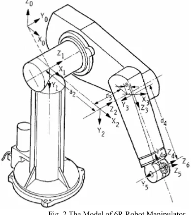
IV. DYNAMIC MODEL OF ROBOT MANIPULATOR A priori information needed for manipulator control analysis and manipulator design is a set of closed form differential equations describing the dynamic behavior of the manipulators. Various approaches are available to formulate the robot arm dynamics, such as Lagrange-Euler, Newton-Euler and Recursive Lagrange [12,13].
[image:3.595.282.550.219.515.2]where
τ
i is generalized torque applied to the system from joint i, L is Lagrangian function (L = K – P, K : total kinetic energy of the manipulator, P : total potential energy of the manipulator),θ
i is the angular position of the joint i, andi
.
θ is the first order derivative of the θi.
Equations which were used for the calculation of the total kinetic energy of the manipulator are given in (27), (28), and (29).
∑
= = 3
1
i i
K
K (27)
∫
= i
i dK
K (28)
(
x y z)
dmdKi i2 i2 i2
2 1
& & & + +
= (29)
[image:4.595.303.549.203.377.2]Equations which were used for the calculation of the total potential energy of the manipulator are given in (30), (31), (32), and (33).
Fig. 2 The Model of 6R Robot Manipulator
Table I. Denavit-Hartenberg Parameters of PUMA 560 Robot Arm
i αi
(degree)
θ
ii a
(meter) i
d
(meter)1 -90 θ1 0 0
2 0 θ2 0.4318 0.1491
3 90 θ3 -0.0203 0
4 -90 θ4 0 0.4331
5 90 θ5 0 0
6 0 θ6 0 0.056
∑
=
= 3
1
i i
P
P (30)
i i
i mgr
P =− 0 (31)
i i i
r
A
r
0=
0 (32)T i i i
i x y z
r =( , , ,1) (33) Where
m
i is the mass of the limb i, g is the gravity vector,i
A
0 is the transition matrix. g =9.8062m/s2.V. SIMULATION RESULTS
In this paper, it was designed 6R (six-DOF) robotic manipulator control using Newton-Raphson (N-R) implemented Generalized Predictive Controller (GPC) algorithm based on joint control. It was compared with RLS (Recursive Least Square) implemented GPC according to the simulation results.
Total simulation time is 10 second and total step number is 10000. In additionally, robot manipulator carries 5 kg load at the end-effecter.
Table II.Some results of simulation robot manipulator by N-R and RLS implemented GPC
Joints Algorithms Initial Angle (rad)
Desired Angle
(rad)
Actual Angle (rad)
Angular Path Error (rad)
N-R 0.0000 0.1745 0.1744 0.0001
Joint
1 RLS 0.0000 0.1745 0.1746 0.0001
N-R -0.0872 0.0000 0.0004 0.0004
Joint
2 RLS -0.0872 0.0000 0.0011 0.0011
N-R 0.3490 0.5235 0.5237 0.0002
Joint
3 RLS 0.3490 0.5235 0.5228 0.0007
N-R -0.3490 -0.1745 -0.1745 0.0000
Joint
4 RLS -0.3490 -0.1745 -0.1745 0.0000
N-R -0.0872 0.3490 0.3491 0.0001 Joint
5 RLS -0.0872 0.3490 0.3480 -0.0020
N-R 0.0000 0.6981 0.6981 0.0000
Joint
6 RLS 0.0000 0.6981 0.6980 0.0010
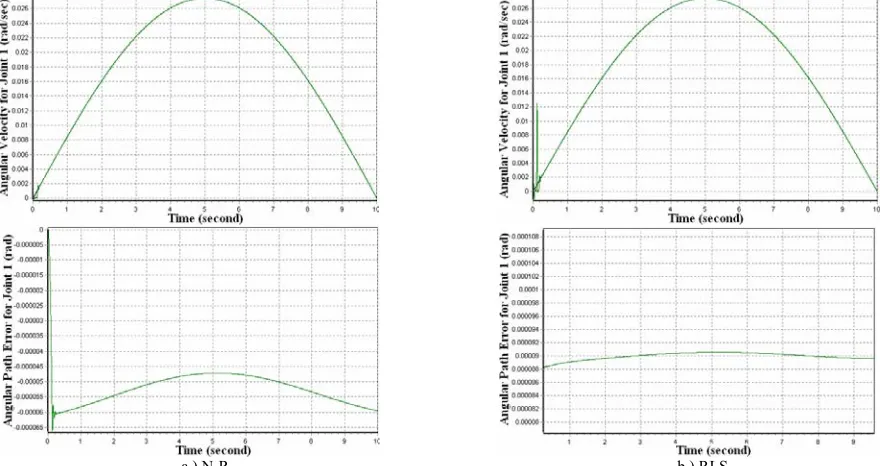
For example, the results of angular path were given in Figure 3. Angular velocities and angular position errors were given belonging to robot arm joint 1, 2 and 5 in Figure 4, 5 and 6 respectively.Additionally, initial- desired-actual angles, angular path errors were given in Table II and also squares of angular velocity error values were given in Table III.
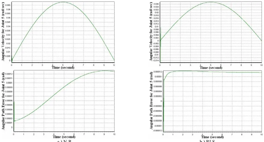
As seen in Table II, angle path errors are smaller in the N-R than those in the N-RLS. On the other hand, the squares of angular velocity errors are proportional to the jerk. The less angular velocity errors at the joints lead to less jerks. With N-R controller happened fewer jolts at the joints.
As seen in Fig. 3, N-R controller tracked to desired trajectory smoother and closer than RLS controller. In tracking performance, both algorithms were found to be satisfactory, according to simulation results of angular velocity given in Figs 4-6. Also, the differences of angular path errors are seen in same Figs.
Table III. Some results of angular velocity errors (rad/sec2)
Joint1 Joint2 Joint3 Joint4 Joint5 Joint6 N-R 0.0000 0.0193 0.0026 0.0000 0.0003 0.000 RLS 0.0016 0.1940 0.0108 0.0004 0.0071 0.001
Table IV. Position errors of robot arm and processing time (CPU’s time) of controllers
Position errors
(mm)
Processing Time (ms)
N-R 0.4772 2625
RLS 0.7681 3469
[image:4.595.50.247.280.498.2]position errors of the N-R controller are lesser than those by RLS. For processing time, simulation of the RLS had taken 3469 ms, whereas the N-R controller has taken 2625 ms, for
the given trajectory Figs 4-6. Newton-Raphson method reduced the time of cost function minimization and also reduced the processing time.
[image:5.595.49.549.98.218.2]
a.) N-R b.) RLS
Fig. 3 Angular Path of Joint 2 by N-R and RLS implemented GPC
[image:5.595.64.526.222.489.2]
a.) N-R b.) RLS Fig. 4 Angular Velocity and Angular Position Errors for Joint 2 by N-R and RLS implemented GPC
[image:5.595.78.518.522.755.2]
[image:6.595.77.518.49.286.2]
a.) N-R b.) RLS Fig. 6 Angular Velocity and Angular Position Errors for Joint 5 by N-R and RLS implemented GPC
In this paper, computationally efficient of cost function minimization in the GPC algorithms was examined. There is over computation in the minimization of the cost function. Newton-Raphson update method requires less iteration numbers for convergence and reduces the calculation
In this application, Recursive Least Square (RLS) implemented GPC between Newton-Raphson implemented GPC controllers were applied to the 6R robot arm manipulator based on joint control. The results of angular path and angular velocity belonging to joints, position error of end-effecter and also processing time of controllers were compared. According to the simulation results, Newton-Raphson implemented GPC reduced position errors and also processing time for robot manipulator control. This means that the Newton-Raphson improved control performance of the GPC.
REFERENCES
[1] J Clarke D W. Application of generalized predictive control to industrial processes. IEEE control Syst. Maga, 1988, 8(2), pp.49-55.
[2] J Richalet, Model predictive heuristic control: Applications to industrial processes, Automatica, 1978, 14(5), pp. 413-428.
[3] Rouhani R., Mehra R K. Model algorithmic control (MAC), Basic theoretical properties, Automatica,1982, 18(4), pp. 401-414.
[4] C R Culter, B L Ramaker, Dynamic matrix control: A computer control algorithm, Proceedings of Joint Automatica Control Conference, San Francisco, 1980.
[5] Köker R., “Design and performance of an intelligent predictive controller for a six-degree-of-freedom robot using the Elman network”, Information Sciences, Volume 176, Issue 12, pp. 1781-1799, 22 June 2006. [6] D. Solaway, P. Haley, Neural generalized predictive contol: a Newton-Raphson implementation, Proceeding of the 11th IEEE International Symposium on Intelligent Control, pp. 277-282, 1996.
[7] G. A. Montague, M.J. Willis, M.T. Tham and A.J. Morris, ”Artificial Neural Network Based Control”, International Conference on Control 1991, Vol. 1, pp.266-271.
[8] Jeong Jun Song and Sunwon Park. “Neural Model-Predictive Control for Nonlinear Chemical Processes”, Journal of Chemical Engineering of Japan, 1993, V26, N4, pp. 347-354.
[9] D.C. Psichogios and L.H. Ungar, ”Nonlinear Internal Model and Model Predictive Control using Neural Networks”, 5th IEEE International
Symposium on Intelligent Control 1990, pp. 1082-1087.
[10] F. Temurtas, H. Temurtas, N. Yumusak, C. Oz, Effects of the Trajectory Planning on the Model Based Predictive Robotic Manipulator Control, Lect. Notes Comput. Sci., 2869 (2003), pp. 545-552.
[11] W.H. Pres, B.P. Flannery, S.A. Teukolsky, and W.T. Vetterling,”Numerical Recipes in C:The Art of Scientific Computing”, Cambridge University Pres 1988.
[12] W. M. Silver, On the Equivalence of Lagrangian and Newton-Euler Dynamics for Manipulators, The International Journal of Robotics Research, Vol. 1(2) (1982) 60-70.
[13] C. S. G. Lee, Robot Arm Kinematics- Dynamics, and Control, Computer, Vol. 15 (12) (1982) 62-80.
![Figure 1 and Table I respectively [14]. In this study,](https://thumb-us.123doks.com/thumbv2/123dok_us/1329580.663875/3.595.282.550.219.515/figure-table-i-respectively-study.webp)