Optimization of a two way MIMO amplify and forward relay network

(1)

R E S E A R C H

Open Access

Optimization of a two-way MIMO

amplify-and-forward relay network

Ying Zhang

1*

, Yinjiang Chen

1

, Chuanyi Pan

1

, Huapeng Zhao

2

and Ning Kang

1

Abstract

In this paper, we consider optimization of a two-way multiple-input multiple-output (MIMO) amplify-and-forward relay network which consists of a pair of transceivers and several relay nodes. Multiple antennas are equipped on the transceivers and relays. Multiple access broadcast scheme which finishes communication in two time slots is considered. In the first time slot, signals received by the relays are scaled by several beamforming matrices. In the second time slot, the relays transmit the scaled signals to the two transceivers. Upon receiving these signals, a MIMO equalizer is implemented at each transceiver to recover the desired signal. In this paper, zero forcing equalizers are used. Joint optimization of the beamforming matrices and the equalizers are realized using the following criteria: 1) the total relay transmission power is minimized subject to the minimal output signal-to-noise ratio (SNR) constraint at each transceiver, 2) the minimal output SNR of the two transceivers is maximized subject to total relay transmission power constraint, and 3) the minimal output SNR of the two transceivers is maximized subject to individual relay transmission power constraint. It is shown that the proposed optimization problems can be formulated as the second-order cone programming problems which can be solved efficiently. The validity of the proposed algorithm is verified by computer simulations.

Keywords: Amplify-and-forward; Beamforming; Multiple-input multiple-output; Relaying; Second-order cone programming; Zero-forcing

Introduction

Relaying technique is capable of extending communica-tion range and coverage by providing link to shadowed users via relay nodes, and it received extensive study in recent years. For collaborative relaying technique, the net-work with a single pair of users and multiple relay nodes equipped with single antenna has been widely investi-gated [1-7]. Zheng [1] assumed perfect knowledge of channel-state information (CSI) and proposed to opti-mize the beamforming vector by maximizing the desti-nation signal-to-noise ratio (SNR) subject to total and local relay transmission power constraints. In [2], sim-ilar optimization criterion was used in the case that only the second-order statistics of CSI are available. In [3,4], quantized CSI was considered. Quantizer at each relay and beamforming vectors at destination were opti-mized to minimize the uncoded bit error rate. In [5],

*Correspondence: [email protected]

1College of Electronic Engineering, University of Electronic Science and Technology of China, Xiyuan Avenue, 610066 Chengdu, China Full list of author information is available at the end of the article

the minimizing mean square error (MMSE) criterion was adopted to optimize the beamforming coefficients. The advantage of this algorithm lies in its ability to adap-tively allocate transmission power of each relay. In recent, a so-called filter-and-forward distributed beamforming technique was proposed in [6]. Different from previ-ous algorithms, this method solved the problem of relay beamforming in frequency selective environments, where a finite impulse response filter is used at each relay. Apart from the above mentioned one-way scheme, a two-way relaying strategy was proposed in [7]. In a two-two-way relaying scheme, the relays cooperate with each other to establish the connection between two transceivers. The design of the beamformer should simultaneously satisfy the requirements from the two transceivers. In [8], an optimization strategy was proposed to optimize the per-formance of a two-way single-input single-output relaying network.

Multiple relay nodes create a virtual multiple-input multiple-output (MIMO) environment at the relay layer.

(2)

With multiple antennas equipped at transmitting and receiving nodes, user nodes can also employ advantages of MIMO techniques, such as spatial multiplexing, space-time coding, and beamforming. Attracted by these mer-its, more and more algorithms are proposed to optimize MIMO relay networks [9-14] and virtual MIMO relay networks [15-18]. Most of these algorithms consider one-way communication scheme, where various optimization criteria are adopted, such as maximizing the destination SNR and minimizing the total system/relay transmission power, MMSE, ZF (zero force), etc. For a single pair of users and multiple relays, a unified algorithm which computes the optimal linear transceivers jointly at the source node and the relay nodes for two-way amplify-and-forward (AF) protocols was proposed [14]. The opti-mization algorithm was designed based on maxiopti-mization of sum rate and MMSE. In [16], a two-way scheme was considered for a relay network with multiple users and single relay. The network was optimized using MMSE criterion at the destination subject to power constraint on relays.

In this paper, we consider a two-way MIMO relay net-work with one pair of transceivers and multiple relays, where the two transceivers are each equipped with M

antennas, and every relay is equipped withN antennas. We assume that relays receive the mixture of signals from two transceivers in the first time slot. With perfect CSI, relays scale the received signals and then transmit these signals to the transceivers in the second time slot. Finally, a MIMO equalizer is used at each transceiver to recover the desired signal. To achieve power-efficient communi-cation, beamforming coefficient matrices are optimized based on three criteria which are designed based on the minimal output SNR and relay transmission power. Mean-while, the MIMO equalizer is optimized by imposing the ZF constraint. It is shown that the proposed optimiza-tion problems can be formulated as the second-order cone programming (SOCP) problems, which can be effi-ciently solved using the cvx toolbox [19]. Contributions of this paper are summarized as follows. First, two-way communication scheme of a MIMO relay network con-sists of multiple relays with multiple antennas is firstly considered. Second,the proposed optimization problem is formulated as an SOCP problem which can be solved efficiently.

The rest of this paper is organized as follows. The ‘Problem formulation’ section presents the problem for-mulation. The ‘Mathematical approximation’ section develops mathematical preparation for optimizing the considered relay network, and ‘Optimization of the proposed relay network’ section gives a detailed optimiza-tion procedure to derive the optimal beamforming and equalization matrices. In the ‘Computer simulations’ section, computer simulations are conducted to

demon-strate validity of the proposed algorithm. Finally, conclu-sions and discusconclu-sions are presented in the ‘Concluconclu-sions’ section.

Notation

Bold lower case is used for vectors, while bold capital let-ters for matrices.Idenotes the unit matrix,∗denotes the complex conjugate operation,Tdenotes the matrix trans-position operation, andHdenotes the complex conjugate transposition operation. tr(A) is the trace of matrix A. vec(A)stacks the columns ofAinto a single column vec-tor.⊗denotes the Kronecker product, and(A0⊕. . .⊕AN) yields a block diagonal matrix with block elements given byAi.

Problem formulation

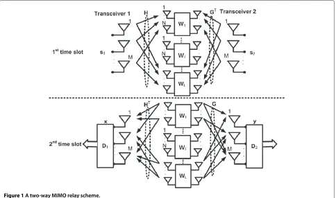
Figure 1 depicts a two-way MIMO relay scheme, where

Wi (i = 1, 2,. . .,L)is the beamforming matrix for the ith relay and Dj (j = 1, 2) is the equalizer for the jth transceiver. Transceiver 1 and transceiver 2 are both equipped with Mantennas. It is supposed that Lrelays equipped with N antennas are used. Flat fading chan-nels are considered. We assume that no direct link exists between the two transceivers. The channel matrix from transceiver 1 to the ith relay is denoted as H_i (i =

1, 2,. . .,L), and the one from theith relay to transceiver 2 is denoted asG_i, whereH_i ∈ CN×M andG_i ∈ CM×N

consist of independent complex Gaussian variables. It is assumed that these channels are reciprocal, i.e., the channel matrix from the ith relay to transceiver 1 is

HT_i , and the one from transceiver 2 to the ith relay is

GT_i . In the first time slot, each transceiver sends mes-sages to theLrelays. With the knowledge of Hi andGi (which can be obtained via training), Wi is computed. In the second time slot, the relays scale the received signals according to Wi and then transmit these sig-nals to the two transceivers. After receiving sigsig-nals, a MIMO equalizer denoted as Dj, j = 1, 2 is used at each transceiver. The aim of this paper is to optimize the performance of the relay network by designing W_i

andD_j.

The mixture of signals received by theith relay can be expressed as

r_i=H_is₁+GT_i s₂+v_i, (1)

where s1ands2 are transmitted signals with covariance

(3)

Figure 1A two-way MIMO relay scheme.

In the second time slot, transceiver 1 and transceiver 2 each receives

x=

L

i=1

HT_iW_ir_i+v_x, (2a)

= L

i=1

HT_iW_iH_is₁+

L

i=1

HT_i W_iGT_is₂

+ L

i=1

HT_i W_iv_i+v_x,

y =

L

i=1

GiWiri+vy (2b)

= L

i=1

GiWiHis1+ L

i=1

GiWiGTi s2

+ L

i=1

GiWivi+vy,

where v_x and v_y denote AGN at transceiver 1 and transceiver 2, and their covariance matrices are assumed to beσ_x2Iandσ_y2I, respectively.s1 ands2are known by

transceiver 1 and transceiver 2, respectively. If Gi, Hi, and Wi are available to transceivers, terms containing

s1 ands2 can be subtracted from Equations 2a and 2b,

respectively. Equations 2a and 2b are then rewritten as

x=

L

i=1

HT_i WiGTi s2+ L

i=1

HT_i Wivi+vx, (3a)

y=

L

i=1

GiWiHis1+ L

i=1

GiWivi+vy. (3b)

A MIMO equalizer is used at each transceiver; thereby, the restored signal after equalization is expressed as

s2=D1x, (4a)

s₁=D₂y. (4b)

Based on Equations 1 to 4, the total relay transmission power and terminal SNRs are defined as follows:

1) Total relay transmission power:

Pr =

L

i=1

EWiri22

(5)

= L

i=1

P1tr

WiHiHHi WHi

+ P2tr WiGTi G∗iWHi

+σ2 vtr

WiWHi

(4)

2) Terminal SNR at transceiver 1:

3) Terminal SNR at transceiver 2:

SNR2=

In subsequent sections,Pr, SNR1, and SNR2will be used

to optimize beamforming matrices and MIMO equalizers.

Mathematical approximation

From (5) to (7), it seems difficult to directly evaluateWi andDjbecause they appear in both signal and noise terms. Therefore, before designing beamformers, three lemmas are derived to makeWiandDjsolvable.

Lemma 1. Total relay transmission power can be ex-pressed as a quadratic function ofw:

Pr=P1wHHw+P2wHGw+σv2wHw, (8)

are defined. The notation ofh_ikandg_ikis given in the proof.

Proof. From (5), the kth column of (WiHi) can be expressed ashT_ik⊗IN

wi, wherehik denotes thekth col-umn of matrixHi. Therefore, the trace of

way of (9) and substituting it and (9) into (5) yield

Pr = P1

Using the definitions in Lemma 1, (8) can be derived.

SNR constraint is usually used in optimizing a relay net-work. For our problem, constraints on destination SNRs are expressed as

SNR1≥γ1, (10a)

SNR2≥γ2, (10b)

whereγ1andγ2 are required SNRs at transceiver 1 and

transceiver 2, respectively. From (6) and (7), it is seen that (10) is related toW_iandD_jin a complicated form. In the rest of this section, two lemmas are derived to transform (10) into a manageable form.

The ZF constraint requires that

D₁

whereD1andD2are defined as the left pseudoinverse of L

i=1HTi WiGTi and L

(5)

Lemma 2. From definitions ofD1andD2given above, if

Proof.It is straightforward to show that

D1DH1 =

Suppose that the eigendecomposition ofH∗HTis given by

In (15), the diagonal ofconsists ofMnonzero eigen-values. The matrixUconsists of all the eigenvectors cor-responding to these nonzero eigenvalues.Uconsists of column vectors which are linearly dependent on columns ofU. The dependence of eigenvectors is caused by rank deficiency ofH∗HTwhose effective rank isM.

We define W = W GT, and assume that W can be represented by the complete orthogonal basis in theNL -dimensional space, whereUis contained in the complete orthogonal basis, i.e., Morthogonal basis of theNL-dimensional space, which can be obtained via Gram-Schmidt procedure based onU.

Substituting (15) and (16) into (14) yields

D1DH1 = H H⊥ U

From (17), it is seen that

tr|DH₁D1

andUconsists of eigenvectors ofGHGcorresponding to its nonzero eigenvalues.

Lemma 3. Inequalities (10) can be relaxed as

σ2

i,hiandQare defined in the following proof.

Proof.With the ZF constraint, (6) and (7) can be

(6)

From the property of tr(.), we may relax the inequality Substituting (18) into (21) yields

SNR1≥

P2M

tr(B)M_i₌₁_|_φ1

ii|2σi

. (22)

From (16) and the definition ofW, we have

= UHW=UHW GT (23)

Therefore, the elements ofcan be represented by

φij=vec(W)H

Similarly, for SNR2, we have

SNR2≥ can be expressed by

φij=vec(W)H

I⊗u∗_ih_j, (26)

whereu_idenotes theith column ofUandh_jdenotes the

jth column ofH. It is assumed that the eigendecomposi-tion ofGHGisUUH.

Similar to Lemma 1, the trace of B and B can be expressed as

tr(B) = σ_v2wHHw+Mσ_x2, (27a) tr(B) = σ_v2wHGw+Mσ_y2, (27b)

where the definitions ofHandGare given inLemma 3.

Substituting (24) and (27a) into (22) and (26), and (27b) into (25) yields

From (28), (10) can be relaxed as

P2M

If every term on the right side of (29a) and (29b) is smaller thanP2

γ1 and

P1

γ2, respectively, i.e.,

P2

(29) can be satisfied.

BecauseWis block diagonal matrices, there are many zero elements in vec(W), which do not contribute to the calculation of (30). SupposeQis chosen such that

w=Qvec(W) (31)

holds.

To derive (30), we have make assumption thatDH₁D₁

andDH₂D₂should be diagonal. From (17), we may achieve this by forcingto be a diagonal matrix. Therefore, the following equations should be satisfied:

φij = vec(W)H

With (30) to (33) and definitions given in Lemma 3, (20) can be derived.

Optimization of the proposed relay network

(7)

Minimizing the total relay transmission power subject to individual minimal output SNR constraint and ZF constraint Using this criterion, the optimization problem is formu-lated as

min

w Pr, (34a)

subject to(SNR1)lower≥γ1, (SNR2)lower≥γ2. (34b)

where (SNR1)lower and (SNR2)lower denote the minimal

output SNR at transceiver 1 and transceiver 2, respec-tively.

Theorem 1. (34) can be approximated as an SOCP prob-lem given as

tor of the left side of (20a) can be represented as

U₂w2₂. Similarly, we defineE_i =

, the nominator of the left side

of (20b) can be represented as U₃w2₂. Using these definitions, (20a) and (20b) can be expressed as

U₂w2₂≤ w

Then, withLemma 3, (35) can be derived.

Maximizing the minimal output SNR of transceivers subject to total relay transmission power constraint and ZF constraint

Assuming that the minimum SNR required by the two transceivers is t, the optimization problem can be formulated as

max

w t, (38a)

subject to(SNR1)lower≥t, (SNR2)lower≥t, Pr≤P. (38b)

where P denotes the maximal total relay transmission power.

(8)

Proof. It can be easily obtained fromLemmas 1to3and

Theorem 1.

Because (39) is quasi-convex, for any given value oft, it becomes the following SOCP problem:

findw, (40a)

subject to (39b) to (39i). (40b)

The bisection search procedure can be applied to solve (40).

Maximizing the minimal output SNR of transceivers subject to individual relay transmission power constraint and ZF constraint

The optimization problem is given as

max

w t, (41a)

subject to(SNR1)lower≥t, (SNR2)lower≥t, (41b)

Pri≤Pi, i=1, ..,L, (41c)

where Pi denotes the maximal transmission power of the ith relay, and Pri = P1tr

WiHiHHi WHi

+ P2tr

W_iGT_i G∗_iWH_i +σ_v2trW_iWH_i .

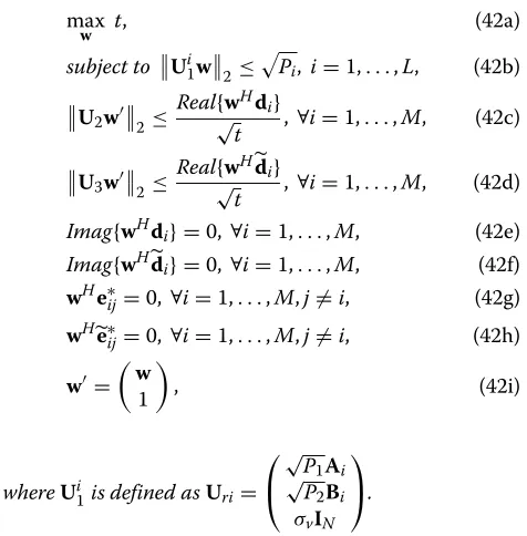
Theorem 3. (41) can be approximated as an SOCP problem:

max

w t, (42a)

subject to Ui₁w₂≤Pi, i=1,. . .,L, (42b) U₂w₂≤ Real{w

H_d i} √

t , ∀i=1,. . .,M, (42c) U₃w₂≤ Real{w

H_d i} √

t , ∀i=1,. . .,M, (42d) Imag{wHdi} =0, ∀i=1,. . .,M, (42e) Imag{wHdi} =0, ∀i=1,. . .,M, (42f)

wHe∗_ij=0, ∀i=1,. . .,M,j=i, (42g)

wHe∗_ij=0, ∀i=1,. . .,M,j=i, (42h)

w=

w

1

, (42i)

whereUi₁is defined asU_ri= ⎛ ⎝

√ P1Ai √

P2Bi

σvIN ⎞ ⎠.

Proof. It can be easily obtained fromLemmas 1to3and

Theorem 1.

For any given value oft, (42) reduces to the following SOCP probelm:

findw, (43a)

subject to (42b) to (42i). (43b)

Similar to the solution of (40), (43) is solved by the bisec-tion search procedure.

Computer simulations

In order to verify the validity of the proposed algorithm, we devise the following simulation scenario. The num-ber of antennas of transceiver 1, transceiver 2, and relays

is assumed to be M = N = 3, and the number of

relays is L = 10. The communication channel coeffi-cients are modeled by complex Gaussian variables with zero mean and varianceσ_h2andσ_g2. The two transceivers transmit independent data streams from different anten-nas with P1 = P2 = 0 dB. AGN on each antenna is

assumed to be complex Gaussian variable with zero mean and unit variance, i.e.,σ_x2 = σ_y2 = σ_v2 = 0 dB. Sources are generated from a QPSK constellation. The values of SNR are computed from 100 independent trials for each plot. Furthermore, the power consumption to increase the minimal output SNR2 for 2 dB becomes smaller as the

value ofγ1increases, which means the derived minimal

output SNR approaches the output SNR as the value of SNR increases. Therefore, less additional power consump-tion is needed to increase the same amount of output SNR. This phenomenon can also be demonstrated by Figure 2.

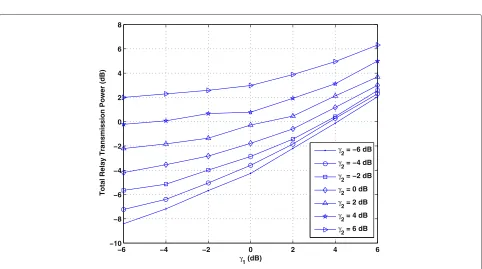
Minimizing the total relay transmission power subject to individual minimal output SNR constraint and ZF constraint We assume thatσ_h2=σ_g2=0 dB. Figure 3 depicts the total relay transmission powerPr against the value ofγ1. It is

observed that the required transmission power increases as the value ofγ1increases. Also, for a givenγ1, the total

relay transmission power increases with the increase ofγ2.

Figure 2 shows the cumulative distribution function (CDF) of the output SNR at transceiver 2 with different values ofγ2. In Figure 2, the value ofγ2is assumed to vary

from−6 to 6 dB with 2 dB stepsize. From the figure, we see that for a givenγ2, the output SNR at transceiver 2 does

not change significantly with the variation ofγ1, and the

output SNR2is about 2 to 3 dB higher than the value of

γ2with 90% probability. This is reasonable since the

pro-posed optimization problem uses the minimal output SNR instead of the real output SNR. It can be seen that the dif-ference between the real output SNR2andγ2decreases as

the value ofγ2increases, which is in accordance with the

phenomenon observed in Figure 3.

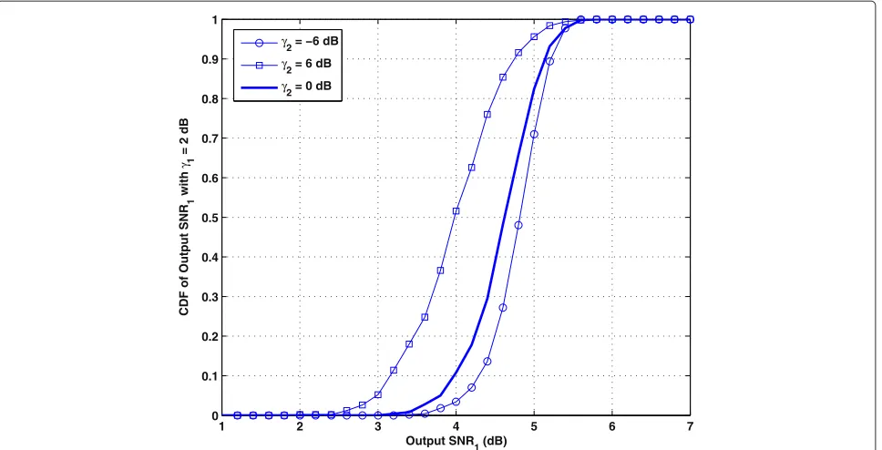
Figure 4 plots the CDF of output SNR1 with different

(9)

−4 −2 0 2 4 6 8 10 12 0

0.1 0.2 0.3 0.4 0.5 0.6 0.7 0.8 0.9 1

Output SNR

2 (dB)

CDF of Output SNR

2

(dB)

γ₂ = −6 dB γ₂ = −4 dB γ₂ = −2 dB γ₂ = 0 dB γ₂ = 2 dB γ₂ = 4 dB γ₂ = 6 dB

Figure 2CDF of the output SNR at transceiver 2 with different values ofγ2.

−6 −4 −2 0 2 4 6

−10 −8 −6 −4 −2 0 2 4 6 8

γ₁ (dB)

Total Relay Transmission Power (dB)

γ₂ = −6 dB γ₂ = −4 dB γ₂ = −2 dB γ₂ = 0 dB γ₂ = 2 dB γ₂ = 4 dB γ₂ = 6 dB

(10)

1 2 3 4 5 6 7 0

0.1 0.2 0.3 0.4 0.5 0.6 0.7 0.8 0.9 1

Output SNR₁ (dB)

CDF of Output SNR

1

with

γ1

= 2 dB

γ₂ = −6 dB

γ2 = 6 dB γ₂ = 0 dB

Figure 4CDF of the output SNR at transceiver 1 with different values of_γ2.

withγ2 = 6 dB is less than that with γ2 = −6 dB. It

is known that Pr is allocated to the relays such that the two transceivers can simultaneously meet the required SNR. It can be concluded from Figure 4 thatPrallocation tends to emphasize maximizing the output SNR which has higher requirement under the condition that the lower SNR requirement can be satisfied. Therefore, SNR1can

achieve a higher average value when γ2 = −6 dB than

whenγ2=6 dB.

Maximizing the minimal output SNR of transceivers subject to total relay transmission power constraint and ZF constraint

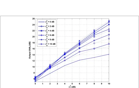
Figure 5 depicts the output SNR at transceiver 1 with the value of σ_h2 changing from 0 to 10 dB. Total relay transmission powers of 0 and 5 dB are considered. It is found that for a given σ_h2, the output SNR1 increases

with the increase of σ_g2, while for a given σ_g2, SNR1

does not keep increasing with the increase of σ_h2. This is because as the quality of channels between transceiver 1 and the relays improves, i.e.,σ_h2increases, the desired transmission power at transceiver 2 to guarantee its out-put SNR increases [2]. Due to limitation of total relay transmission power, the output SNR at transceiver 1 can not increase consistently. When the quality of channels between transceiver 2 and the relays improves, the output SNR1increases with the increase ofσ_h2.

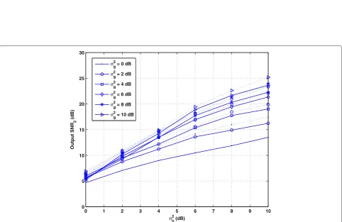
Figure 6 shows the same plot for output SNR2. It is

observed that the output SNR2increases with the increase

ofσ_h2, it while does not increase with the increase ofσ_g2 especially whenσ_g2 is high andσ_h2is relatively low. The reason is the same as that for SNR1versus σ_h2. Also, as

noticed from Figures 5 and 6, the output SNR1and SNR2

increases with the increase of the total relay transmission power.

Maximizing the minimal output SNR of transceivers subject to individual relay transmission power constraint and ZF constraint

In this simulation, we assume that the total relay transmis-sion power is uniformly allocated to the relays. Figures 7 and 8 show the output SNR versus the value of σ_h2 with individual relay powers of−10 and 0 dB. It is noted that these plots are similar to those with total relay transmis-sion power constraint. With the increase of individual relay transmission power, output SNRs at transceiver 1 and transceiver 2 increase. Compared with Figures 5 and 6, it is found that the output SNR1and SNR2are slightly

lower with individual power constraint than those with total power constraint. This is because individual power constraint is more restrictive than the total power con-straint.

Conclusions

(11)

Figure 5OutputSNR1versus the value ofσ_h2.Solid line: with total relay transmission power of 0 dB, dash line: with total relay transmission power of 5 dB.

Figure 6OutputSNR2versus the value ofσ_h2.Solid line: with total relay transmission power of 0 dB, dash line: with total relay transmission power

(12)

0 1 2 3 4 5 6 7 8 9 10 5

10 15 20 25 30

σ_h2 (dB)

Output SNR

1

(dB)

σg 2

= 0 dB

σ_g2_{= 2 dB} σ_g2

= 4 dB

σ_g2_{= 6 dB} σ_g2

= 8 dB

σ_ga_{= 10 dB}

Figure 7OutputSNR1versus the value ofσ_h2.Solid line: with individual relay transmission power of−10 dB, dash line: with individual relay

transmission power of 0 dB.

0 1 2 3 4 5 6 7 8 9 10

0 5 10 15 20 25 30

σ_h2_(dB)

Output SNR

2

(dB)

σ_g2 = 0 dB

σ_g2_{= 2 dB} σ_g2

= 4 dB

σ_g2_{= 6 dB} σ_g2

= 8 dB

σg 2

= 10 dB

Figure 8OutputSNR2versus the value ofσ_h2.Solid line: with individual relay transmission power of−10 dB, dash line: with individual relay

(13)

efficiently. Computer simulation demonstrates validity of the proposed algorithm. Furthermore, it is straightfor-ward to see that the proposed algorithm can be imple-mented distributively as long asUandUare broadcasted to all the relays. With w replaced by wi, U1 replaced

byUri,U2 replaced by

σvCi 0

0T σx

, and U3replaced by

σvDi 0

0T σ_y

, (35), (39), and (42) can be solved at each

relay. The performance of distributed implementation will be analyzed in our future work.

Competing interests

The authors declare that they have no competing interests.

Acknowledgements

The author wishes to acknowledge the financial support of the National Science Foundation of China through Grant No. 61101094 and No. 61201275.

Author details

1_{College of Electronic Engineering, University of Electronic Science and}

Technology of China, Xiyuan Avenue, 610066 Chengdu, China.2_Department

of Electronics and Photonics, Institute of High Performance Computing, Fusionopolis Way, Singapore 138632, Singapore.

Received: 12 May 2014 Accepted: 8 December 2014 Published: 30 December 2014

References

1. G Zheng, Collaborative-relay beamforming with perfect CSI: optimum and distributed implementation. IEEE Signal Process Lett.16(4), 257 (2009) 2. V Havary-Nassab, S Shahbazpanahi, A Grami, Z-Q Luo, Distributed

beamforming for relay networks based on second-order statistics of the channel information. IEEE Trans. Signal Process.56(9), 4306 (2008) 3. MM Abdallah, HC Pagadopoulos, Beamforming algorithms for

implementation relaying in wireless sensor networks. IEEE Trans. Signal Process.56(10), 4772 (2008)

4. E Koyuncu, Y Jing, H Jafarkhani, Distributed beamforming in wireless relay networks with quantized feedback. IEEE J. Selected Areas Commun.

26(8), 1429 (2008)

5. N Khajehnouri, AH Sayed, Distributed MMSE relay strategies for wireless sensor networks. IEEE Trans. Signal Process.55(7), 3336 (2007) 6. H Chen, AB Gershman, S Shahbazpanahi, Filter-and-forward distributed

beamforming in relay networks with frequency selective fading. IEEE Trans. Signal Process.58(3), 1251 (2010)

7. V Havary-Nassab, S Shahbazpanahi, A Grami, Optimal distributed beamforming for two-way relay networks. IEEE Trans. Signal Process.

58(3), 1238 (2010)

8. H Chen, Beamforming Optimization for Two-Way Relay Channel (2014). p. 28–31

9. Y Rong, Optimal joint source and relay beamforming for MIMO relays with direct link. IEEE Commun. Lett.14(5), 390 (2010)

10. B Khoshnevis, W Yu, R Adve, Grassmannian beamforming for MIMO amplify-and-forward relaying. IEEE J. Selected Areas Commun.

26(8), 1397 (2008)

11. W Guan, H Luo, Joint MMSE transceiver design in non-regenerative MIMO relay systems. IEEE Commun. Lett. J.12(7), 517 (2008)

12. Y Rong, F Gao, Optimal beamforming for non-regenerative MIMO relays with direct link. IEEE Commun. Lett. J.13(12), 927 (2009)

13. AS Behbahani, R Merched, AM Eltawil, Optimization of a MIMO relay network. IEEE Trans. Signal Process.56(10), 5063 (2008)

14. K-J Lee, H Sung, E Park, I Lee, Joint optimization for one and two-way MIMO AF multiple-relay systems. IEEE Trans. Wireless Commun.

9(12), 3671 (2010)

15. A El-Keyi, B Champagne, Adaptive linearly constrained minimum variance beamforming for multiuser cooperative relaying using the Kalman filter. IEEE Trans. Wireless Commun.9(2), 641 (2010)

16. J Joung, AH Sayed, Multiuser two-way amplify-and-forward relay processing and power control methods for beamforming systems. IEEE Trans. Signal Process.58(3), 1833 (2010)

17. R Zhang, C Choy Chai, Y-C Liang, Joint beamforming and power control for multiantenna relay broadcase channel with QoS constraints. IEEE Trans. Signal Process.57(2), 726 (2009)

18. O Oyman, AJ Paulray, Design and analysis of linear distributed MIMO relaying algorihms. IEEE Proc. Commun.153(4), 565 (2006) 19. M Grant, S Boyd, cvx user’s guide for cvx version 1.21 (build 790).

http://cvxr.com/cvx/. Accessed 16 July 2013

doi:10.1186/1687-6180-2014-184

Cite this article as:Zhanget al.:Optimization of a two-way MIMO amplify-and-forward relay network.EURASIP Journal on Advances in Signal Processing20142014:184.

Submit your manuscript to a

journal and beneﬁ t from:

7Convenient online submission 7Rigorous peer review

7Immediate publication on acceptance 7Open access: articles freely available online 7High visibility within the ﬁ eld

7Retaining the copyright to your article