R E S E A R C H
Open Access
Localization of ambiguously identifiable
wireless agents: complexity analysis and
efficient algorithms
Stephan Schlupkothen
*and Gerd Ascheid
Abstract
In the localization of wireless agents, ambiguous measurements have significant implications regarding the complexity and quality of the agents’ positioning. Ambiguous measurements occur, for example, inmultiple source localization (MSL), in which the goal is to localize the sources of signals, although the signals themselves cannot be used to differentiate among their sources. The indifferentiability of the sources results in a combinatorial optimization problem that must be solved before a localization result can be obtained. Similar effects arise, for example, in the localization of highly resource-limited wireless agents that are subject to severe size and energy constraints, meaning that neither unique identification sequences (CDMA) nor unique frequency or time resources (FDMA, TMDA) can be used. This application scenario constitutes a more general and complex joint problem of localization and ambiguity resolution that also encompasses MSL. In this work, we focus on this more general problem and its corresponding application case while maintaining applicability to the MSL problem. More precisely, we prove theN P-hardness of the joint localization and ambiguity resolution problem and derive a solution framework that facilitates a
comprehensive and concise formulation thereof. Thereby, we derive a minimum mean square error (MMSE)-optimal algorithm based on mixed-integer nonlinear programming and propose a relaxation of the problem with the aim of reducing the computational complexity. Additionally, simplifications are derived for the case in which bidirectional measurements are available or enforced, e.g., by the applied communication or ranging protocol.
Keywords: Wireless sensor networks, Localization, Transmit ambiguities
AMS subject classification: 90C35; 90C26; 90C27; 90C59; 90C11
1 Introduction
The unique identification of users and agents in wireless networks is generally regarded as a design requirement. Particularly in networks in which the localization of the network participants is essential, non-unique identifica-tion is known not only to complicate the localizaidentifica-tion process but also to significantly impact its quality. How-ever, in some application scenarios, unique identification is inherently impossible or is prevented by highly restric-tive size and energy constraints imposed on the wireless autonomous agents. Two examples of such scenarios are detailed in the following. These examples emphasize the significance and importance of localization algorithms
*Correspondence:[email protected]
Chair for Integrated Signal Processing Systems, RWTH Aachen University, Templergraben 55, Aachen, Germany
that are able to cope with non-unique measurements, for joint localization and ambiguity resolution in particular.
Application Case 1 (Multiple source localization (MSL) In MSL, the goal is to l on the signals they emit. These signals do not include any identification information that reveals information about their original sources. Hence, stations that receive these signals cannot differentiate among their sources, which prevents the use of classi-cal loclassi-calization algorithms. This scenario is illustrated in Fig.1and described in more detail in Section2.1.1.
Application scenarios of MSL include the following:
• The localization of, e.g., pedestrians using privacy-preserving techniques such as ultrasound
• Passive localization of flying objects
• Gunshot detection, e.g., in public areas
Fig. 1MSL scenario with two sources and four stations that forward the measured data to a fusion center that localizes the sources. The stations cannot distinguish between the two sources, as visualized by black, i.e., non-colored signals
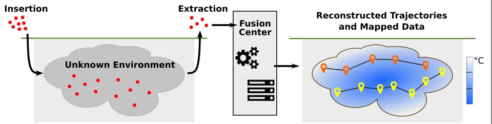
Application Case 2 Emerging application scenarios for miniature wireless agents include the exploration of secluded and difficult-to-access environments such as subterranean cavities or pipelines. Examples include oil reservoirs, which have recently been shown to be of sig-nificant economical and academic interest [1,2]. Related industrial applications include oil extraction using the cold heavy oil production with sand (CHOPS) technique, in which sand-free channels of varying diameters, ranging from one to several centimeters, and of several hundred meters in length are created [1, 3]. Because of the high salinity of the environment [4], the use of typical radio-frequency transmitters is unattractive [5]. Hence, the use of ultrasound is being considered for communication among the agents as they traverse these channels.
Wireless agents equipped with environmental sen-sors1 are currently the most promising candidates for gathering interesting data from such an environ-ment to answer questions regarding, e.g., the system’s temperature, pressure, or fluid composition distribution.
The corresponding exploration procedure is illustrated in Fig. 2. However, in such application scenarios, particu-larly severe constraints are imposed on the agents. Typical examples of such constraints are listed below:
• Size constraint: An initial feasibility study reported in [1] revealed that millimeter-sized agents are needed to successfully pass through such an environment, as larger agents are destroyed during injection or cannot be recovered2.
• Energy budget: Due to the size constraint, the energy available for, e.g., communication and sensing, is inherently limited. Moreover, an operation time of up to 48 h has been shown to be required [1], which demands further energy savings.
• Swarm size constraint: Due to the spatial extent of the environment and the limitations of each individual agent with respect to its energy, communication range, and sensing capabilities, thousands of agents are required to compensate for
these limitations such that sufficient data on all areas in the environment can be collected.
• Localizability: To properly utilize the measurements made by the agents, localization of the agents is required. Because secluded and difficult-to-access environments generally do not permit positioning using GPS, pairwise distance measurements—e.g., by means of two-way ranging—are conducted. Because of the swarm size constraint and the generally strict energy limitations, significant limits must be imposed on the energy that can be spent for, e.g.,
communication to ensure that ranging can be performed with any arbitrary agent, which is required because of the decentralized nature of the network. Hence, all agents in the swarm must share the same time/frequency resources.
For successful exploration, a trade-off must be estab-lished between the agents’ capabilities and resource con-sumption. Inspired by the general feasibility of using measurements to localize wireless agents that are not uniquely identifiable–cf. Application Case 1 (the MSL case)–the use ofsharedcommunication resources is pro-posed. Specifically, the use of Direct-Sequence Code Divi-sion Multiple Access (DS-CDMA) for channel access is proposed, in which non-unique DS-CDMA codes are used to significantly reduce the energy consumption of the agents. In this way, the following benefits are achieved:
• The energy consumption per ranging pulse is reduced. Instead of2N bits, whereN is the number of agents in the swarm, only2K(K < N) bits are used in the DS-CDMA sequence, thereby reducing the energy consumed for transmission and reception.
• Less memory is needed for storage, and less logic is needed for correlating the received DS-CDMA sequences.
• Reductions are achieved in both the signal pulse length and multi-path effects. Multi-path effects are induced by, among other factors, the narrowness and reflectivity of the environment.
Note that the burden imposed by the main disadvantage of this approach, i.e., the increased localization complex-ity, is shifted to the fusion center, where offline position-ing is performed after the agents have been extracted from the environment and where sufficient computational resources are available.
Conclusion Consequently, in both application cases, the following interrelated problems must be solved:
1. The transmit ambiguities (TAs) in the distance measurements must be resolved, i.e., it is necessary
to find a mapping between the distance
measurements and the agents that recorded them. 2. The agents must be localized, i.e., the positions of the
agents must be estimated based on their distance measurements.
To address both problems simultaneously, algorithms are needed that can jointly resolve the ambiguities and localize the agents. Such algorithms are key enablers for the application cases described above. In the following, this joint problem is called the joint localization and trans-mit ambiguity resolution problem (JLTAP). This work presents a thorough analysis of this problem and the derivation of the governing constraints as well as the formulation of both optimal and sub-optimal solutions.
1.1 Related work
The MSL problem has been under study for several years, e.g., in [6–8]. However, neither a thorough graph-theoretical analysis nor a formulation of a minimum mean square error (MMSE)-optimal or maximum like-lihood (ML)-optimal algorithm has yet been presented. For example, the authors of [6] considered time-of-arrival (TOA)-based measurements and proposed a heuristic solution consisting of the following three steps:
• Coarse localization of the sound sources. In this step, important governing equations are ignored.
• Sub-optimal TA resolution, i.e., estimation of the mapping between the TOA measurements and the sound sources. In this method, non-convex terms are replaced with local linearizations.
• Refinement of the sound source localization result.
However, because the authors of [6] considered time instead of distance measurements, their algorithms and methods are not directly applicable to the scenarios con-sidered in the present work.
The more general problem arising from non-unique communication identifiers, e.g., for miniature agents, was first studied by Duisterwinkel et al. in [9]. These authors considered the case in which several agents are assigned to the same OFDM sub-carrier, thus resulting in non-unique identification. To address the localization chal-lenges posed by this scenario, a heuristic based on dif-ference thresholding was applied, in which two distance measurements were considered to have been recorded by agent i with respect to agent j and vice versa if |mk→j − ml→i| ≤ .
approach targets only the resolution of the TAs and does not jointly address the localization problem.
More recently, Duisterwinkel et al. [13] presented a ran-dom sample consensus (RANSAC)-based algorithm using the difference thresholding technique introduced above. Consequently, the algorithm reported in [13] requires bidirectional measurements.
The classical ML-optimal agent localization problem, i.e., in the absence of any TAs, is known to be non-convex in general [14]. Moreover, the authors of [15] have shown that the localization problem for sparse net-works and in the absence of TAs and measurement noise isN P-hard. The first algorithms to focus on improving the computational feasibility of this problem via convex relaxations were based mainly on semi-definite program-ming (SDP), as in [16–20], and second-order cone pro-gramming (SOCP) [21]. Further SDP-based relaxations, e.g., the so-called edge-SDP relaxation, have also been derived to reduce the computational burden [22]. Further-more, a computationally efficient multi-dimensional scal-ing (MDS) algorithm [23] and a matrix-completion-based approach [24] have been proposed. A global-continuation and least-squares formulation has been investigated, e.g., in [25]; such formulations are especially interesting for the localization of many agents because these algo-rithms are less resource-demanding than SDP and SOCP formulations.
1.2 Our contributions
Our contributions in this work are fourfold. First, we present a framework that facilitates the concise formula-tion of the problems corresponding to both considered application cases, and this framework is also used to illus-trate that MSL is a special case of the more general JLTAP. Second, we show that the JLTAP isN P-hard by means of a Karp reduction. Third, an MMSE-optimal algorithm is presented that is based on mixed-integer nonlinear pro-gramming (MINLP) and does not require bidirectional measurements. Finally, a sub-optimal algorithm is derived from the MINLP formulation to mitigate the exponential worst-case complexity of the optimal algorithm.
1.3 Organization
The remainder of this work is organized as follows: Section2introduces the general system model as well as the corresponding assumptions and the notation used. It also highlights the similarities between the two considered application cases. In Section 3, the governing equations for TA resolution and agent or source localization are derived and combined to formulate the optimal JLTAP algorithm. The results are used in Section 4 to derive and motivate a relaxed, sub-optimal algorithm. Numeri-cal results and the simulation environment used to obtain them are presented in Section5. In Section6, conclusions
are drawn and future work is outlined. TheN P-hardness of the JLTAP is proven in Appendix 1.
2 System model and problem formulation
Following the general methodology outlined in Section1 and visualized in Fig.2, the agents use their omnidirec-tional antennas to perform ranging with all nearby agents in their communication range, which is represented by a radiusR.
It is assumed that each agent has a unique serial number (SN) and a transmission code (henceforth called a trans-mit ID, or simply an ID). Moreover, it is assumed that the SN is accessible only through physical access to the agent, whereas the ID is used by the agent for communi-cation, e.g., a DS-CDMA sequence. Hence, when an agent transmits an ultrasonic pulse (ranging pulse), the receivers are aware only of the transmitter’s ID. The mapping from SNs to IDs is fixed and known only to the fusion center. Based on the transmitted ranging pulses, distance mea-surements can be performed, whose inaccuracy can be modeled as additive Gaussian noise3:
dj→i=di,j+ni,j, (1)
whereni,j∼N
0,σij2is an independently and identically distributed (iid) Gaussian noise variable with varianceσij2,
di,jdenotes the actual distance between agentsiandj, and
dj→i is the random variable (RV) that describes the
dis-tance measured by agentibased on a ranging pulse sent by agentj.
In the following, we usem•→ito denote actual
measure-ments, i.e., realizations of the corresponding RVs, where • serves as a placeholder, and we useMIJ→i to denote
the tuple of all measurements recorded by agent i with respect to agents using ID IJ. In the case that agents i
andj∈S(IJ)are out of communication range, the corre-sponding non-existent measurement is represented by∞ in the measurement tuple.
Because of the large number of agents, the continuous introduction thereof into the environment, and the long time required until the first agents reach the extraction point4, it is believed that the computationally intensive tracking of all agents can be replaced with a single local-ization computation whenever the swarm is distributed throughout the entire environment.
2.1 Notation and problem formulation
Fig. 3Illustration of the notation used in this paper and the effects of TAs. Consider an agenti, which is assumed to use IDIR(red) and two nearby agents (which use IDIB(blue)), one of which is within the communication range (denoted byR) ofi. The actual distances between the pairs of agents and the RVs that describe the possible measurements of these distances are illustrated. For the two cases, the table on the right-hand side clarifies both the notation and the fact that no distance measurement is made betweeniandk. Here,m˙∼dis used to denote that the measurement
mis a single realization, i.e., sample, of the distributiond
the ranging pulses corresponding to the various mea-surements are not known. Therefore, resolving the TAs means solving the mapping problem between the set of measurements MIJ→i and the set of RVs DIJ→i =
dk
j→i|j∈S(IJ),k∈N
. More precisely, each measure-ment needs to be mapped to an RV subject to certain constraints, which will be derived in Section3.
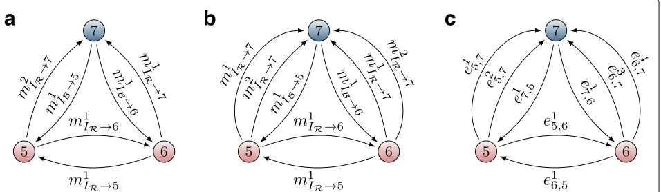
An example network in which TAs arise is depicted in Fig.4a, where two agents (“5” and “6”) both use IDIR(red) and a third node (“7”) usesIB(blue). Node “7” receives two ranging pulses from the other two nodes. Based on these pulses, it measures the ranges m1I
R→7andm2IR→7
. Because of the TA, it cannot uniquely relate the measured ranges to the physical agents S(IR), and hence, local-ization using classical methods such as those discussed in Section 1.1 is not possible. Henceforth, the follow-ing formal definition will be adopted for the problem at hand.
Definition 1(Joint localization and transmit ambigu-ity resolution problem (JLTAP))In the JLTAP, the objective is to jointly estimate the Cartesian position of each agent based on the obtained range measurements. Inherently, it is necessary to resolve the TAs, i.e., to find a mapping
between each measurement mkIJ→
iand the corresponding
agent l∈S(IJ)such that mkI
J→iis a realization of the RV
dl→i.
A corresponding mathematical description, including the formulation of an optimization problem, is derived in Section3.1.
2.1.1 Relationship with MSL
In MSL, the objective is to localize sources based only on the signals they emit. An example scenario is illus-trated in Fig.1, where two sources emit sound signals that are received by nearby stations. Because the stations can-not differentiate between the two different sources of the
a
b
c
Fig. 4 aIllustration of a network in which two agents (“5” and “6”) are using the same ID. The edges are annotated with the corresponding measurements of the ranging pulses. This graph is also called thetrue graph.bGraph showing theeffectiveambiguities due to the TAs. Here, additional edges are introduced to account for all potential origins. The edges are annotated with their weights.cGraph showing the labels or
namesof the edges that match the variable notationxk
ijintroduced in Section3.1.2. Note that the order of the superscript numbering is arbitrary. Example,WA
signals they receive, the fusion center, which has access to the measurements from all stations, must resolve the ambiguities in the measurements and perform the local-ization. Consequently, the MSL problem is closely related to the problem considered in this work. However, the fol-lowing assumptions are usually adopted in the case of MSL (see, e.g., [6]):
i) The sensitivities of the stations and their positions are such that every station can receive signals from all sources. Consequently—unlike in the case of wireless agent localization—the measurements consist only of direct distance measurements between the stations and the sources. This generally reduces error propagation during localization and simplifies the problem formulation, as out-of-range agents do not need to be considered.
ii) The number of stations and their positions are such that the conditions for good localization (see, e.g., [26,27]) are fulfilled once the ambiguities have been resolved.
iii) There are significantly fewer sound sources in the case of MSL than there are wireless agents in the application case considered in the present work. Therefore, the complexity of the ambiguity resolution problem is significantly lower in the MSL case. iv) Only one kind of source is considered. This is
equivalent to the assumption that all sources use the same transmit ID.
Items i) and iv) in particular render MSL algorithms inapplicable for the more general problem considered in this work (cf. Application Case 2).
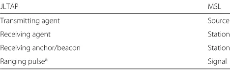
A high-level comparison between the two problems cor-responding to the two considered application cases is presented in Table1.
3 MMSE-optimal JLTAP formulation
This section is divided into two main parts. The first, Section 3.1, covers the derivation of the mathematical formulation of the TA resolution problem. The second, Section 3.2, covers the incorporation of the localization
Table 1Analogies between agent localization and MSL
JLTAP MSL
Transmitting agent Source
Receiving agent Station
Receiving anchor/beacon Station
Ranging pulsea Signal
aNote that whereas the ranging pulses in the JLTAP can include different transmit
IDs and ambiguities arise only with respect to agents using the same ID, allsignalsin the MSL problem are assumed to be of the same kind; this assumption is analogous to the use of a single ID in the JLTAP
problem to obtain the joint optimization formulation of the JLTAP.
3.1 Part I: derivation and properties of the TA resolution formulation
Based on the assumptions stated in Section1, the follow-ing graph-theoretical representation is used:
1) Every agent is modeled as a vertex of a graph, i.e., agenti corresponds to vertexvi∈VT.
2) Every measurement is represented by a directed edge fromvjtovi,eji = (vj,vi)∈ET, whereviis the agent
that recorded the measurementmj→iassociated with
this edge.
3) Every edge in the graph has a corresponding weight W(eji) = mj→i, which is equal to the value of the
associated distance measurement.
Henceforth, this graph is called the true graph (TG),
GT = (VT,ET,WT), because its representation
inher-ently assumes that either no TAs have arisen or all TAs have been resolved. An example is given in Fig. 4a. For simplicity of description, a graph-theoretical view is adopted, in the sense that the origin of a measurement
mj→i(and edgeeji) is considered to be agent or vertexj,
whereas the termtargetis used to refer to agent or vertex
i, which actually measured the distance.
3.1.1 Problem analysis
To derive the solution to the TA resolution problem, the following observations are considered:
4) For every measurementmkIJ→i, every agent in S(IJ)is a potential origin candidate.
5) The solution to the TA resolution problem should consist of exactly one unique mapping, i.e., exactly one origin for each measurement. 6) Between each pair of vertices, there can be at most one edge in each direction, i.e., at most one edgee = (vi,vj)and at most one edge
e = (vj,vi).
An example of the TA-aware graph representation is shown in Fig.4b, and this representation is subsequently referred to as the ambiguity graph (AG). Note that this graph is generally a directed multi-graph. The AG is denoted byGA = (VA,EA,WA)and is defined as follows:
7) The vertices correspond to agents in the network. 8) For each measurementmkIJ→i, a directed edge with a
weight ofmkI
J→iis drawn betweenviand each
vj(j∈S(IJ)). Edges of this kind are henceforth referred to ascopies of both each other and the corresponding measurement. Consequently, there are|S(IJ)|directed edges with a weight ofmkI
3.1.2 Mathematical formulation
From the descriptions provided above, it can be under-stood that the problem of resolving the TAs is a special kind of decision or selection problem. Consequently, the mathematical formulation will include binary decision variables with the following constraints:
9) For each edge in the AG, a binary decision variable denoted byxkji∈ {0, 1}is introduced. This variable will be equal to one iff the corresponding edge, i.e., the measurementmkIJ→i, is selected to represent the mapping of a measurement made by agenti to a ranging pulse from agentj.
10) Once an edgemk
IJ→ihas been selected, allcopies of
that edge, i.e., those that were created due to Item 8, can no longer be selected. Consequently, the sum of the corresponding decision variables is constrained to be exactly one.
11) Because the static case is considered, at most one measurement may be selected from among all parallel5edges between two vertices. This is necessary because copy edges, cf. Item 8, are drawn between all possible vertices and full connectivity is not necessarily guaranteed. Consequently, the sum of all corresponding decision variables is constrained to be at most one.
Thus, the following feasibility problem, which considers only the resolution of the TAs, can be formulated. In the following subsection, this problem will be extended to the complete JLTAP by incorporating the joint consideration of the localization problem. Item 8),Pi,jis the set of all parallel edges directed from
vertexito vertexj, andxkijis the decision variable corre-sponding to edgeek
ij. Note that constraints (2c) and (2d)
arise directly from the description of the AG (cf. Items 8, and 10). Item 11 is accounted for by constraints (2e) and (2f), which both account for parallel edges.
RemarkAlthough constraints (2e) and (2f) are
redun-dant, they are explicitly mentioned in Eq.(2)because
simu-lations have shown that their explicit formulation enables significant reductions in computational complexity.
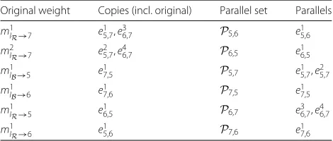
For the example depicted in Fig.4, the copy sets and parallel sets are given in Table2.
3.2 Part II: TA-free wireless agent localization and JLTAP formulation
The objective of agent localization is to obtain the Carte-sian positionspi = (px,i,py,i) orpi = (px,i,py,i,pz,i)
of all agents i ∈ V from noisy distance measurements (cf. Eq. (1)). The matrix of all agent positions is denoted by P = p1,. . .,p|V|. Because of the assumption of iid additive Gaussian noise, the corresponding ML objec-tive function for the localization problem can be easily derived [28]:
Note that this problem is known to be non-convex in general [14]. For simplicity, it is assumed that all noise variances are equal, i.e.,σij = σ ∀(vi,vj)∈E.
3.2.1 Integration into the JLTAP
To obtain a joint problem formulation that includes both localization and TA resolution, which requires combin-ing the objective function given in (3) with the feasibility problem expressed in (2), the following issues must be resolved:
12) Due to the TAs and the joint approach, the particular measurementsmj→ito be used in (3) are not known
because the decision problem regarding their mapping has not yet been solved.
13) In the AG that serves as the basis for solving the JLTAP, edges exist for all possible candidates. However, in (3), only those pairs of vertices(vi,vj)to
which a measurement is currently assigned should be considered.
Table 2Copy and parallel sets for the example in Fig.4
Original weight Copies (incl. original) Parallel set Parallels
To accommodate these constraints, the objective func-tion given in (3) is modified as follows:
whereWA(ekij)denotes the weight (measurement value) of
edgeekijin the AG (cf. Fig.4) and allxkijare the same binary decision variables as in (2).
In this expression, the sum in the inner brackets will select the measurements to be used and– in conjunc-tion with further constraints– ensure that at most one measurement per link is chosen (cf. Item 12. The sec-ond sum, which is newly introduced here, ensures that the case in which no measurement is selected is also handled correctly (cf. Item 13.
3.3 Synthesis and NP-hardness
This section combines the results from the previous Sections 3.1and 3.2to obtain the MMSE-optimal for-mulation of the JLTAP. Moreover, an extension of the joint formulation expressed in (5) is presented that facilitates faster and more accurate solutions in the case that bidi-rectional measurements are available or corresponding solutions should be enforced.
Based on the results obtained in Sections3.1and 3.2, the MMSE-optimal JLTAP formulation can be expressed as follows:
where the objective function represents the residual local-ization error and the constraints arise from the TA reso-lution conditions.
Note that this problem is a MINLP problem. In Appendix1, we prove that solving Problem (5) requires solving a problem that is N P-hard in general. For this
reason, a relaxation of this problem is introduced in the following section.
3.3.1 Applicability to MSL
As outlined in Section2.1.1, MSL can be regarded as a special case of the JLTAP, and thus, Problem (5) can also be used to describe MSL problem instances. To this end, it should be noted that in MSL, all sources have the same ID. Consequently, copy edges are introduced among all sources, and the set of parallel edges is easily deducible. However, a formal simplification of Problem (5) for the case of MSL is generally not possible.
3.3.2 Enhancements for bidirectional measurements
In the case that bidirectional measurements are guaran-teed or corresponding solutions should be enforced, addi-tional constraints can be introduced. These constraints reduce the search space and have thus been shown to significantly reduce the run-time and memory demands placed on solvers.
The constraints are given as follows:
solution candidates exist that can fulfill the bidirectional-ity criterion. Similarly,Bdenotes the set of vertex pairs for which this is not the case.
4 JLTAP relaxations
To mitigate the difficulties caused by the non-convexity, N P-hardness, and general computational complexity of the optimal JLTAP algorithm presented in Section3.3, this section introduces a relaxation of the JLTAP problem. The purpose is to make the original problem more numerically tractable while requiring only minor modifications to the objective function and the constraints.
The following approximations and simplifications are adopted:
• The binary constraint (5b) is replaced with a continuous interval constraint, i.e.,xkij∈[ 0, 1]is substituted forxkij∈ {0, 1}. In this way, all discrete optimization variables are replaced with continuous variables, which eliminates the need for discrete solvers.
• The constraint corresponding to Item 13 is loosened, i.e., the equality constraintqij = kxkijis replaced
with the inequality constraintqij ≥ kxkij. In
simulations not reported in this work, this relaxation has been shown to yield improved convergence and accuracy. Details regarding the non-convexity of the relaxed JLTAP without this relaxation can be found in Appendix2.
Thus, the following optimization formulation of the relaxed, sub-optimal JLTAP is obtained:
arg min
Note that the objective function–and hence Problem (7)–is still non-convex, although a dedicated integer pro-gramming solver is no longer required. Consequently, classical interior-point solvers can ensure only locally optimal solutions. Due to the joint approach, the positions of the agents are also directly estimated, meaning that a reversal of the relaxation– i.e., a mapping from the contin-uousxkij ∈[ 0, 1] to the binary variablesxkij ∈ {0, 1}– is not required.
5 Numerical results and discussion
In this section, numerical results obtained using the devel-oped algorithms are presented and discussed.
5.1 Method
The Monte Carlo simulation results presented in the fol-lowing subsections were obtained as follows:
• The data collected by the agents distributed in the environment were simulated (cf. Section5.2).
• The data processing performed by the fusion center (cf. Fig.2) was simulated to evaluate the proposed algorithms using the simulated agent measurements.
• A performance comparison of the algorithms was performed using the metric defined in Section5.3.
All simulations were performed using MATLAB and the BARON solver [29].
5.2 Simulation environment
Simulations were performed by randomly placing N
agents in the two-dimensional unit box [−0.5, 0.5]2 fol-lowing a uniform distribution. To ensure that the IDs were assigned to the agents as equally as possible, the following procedure was used: First,NIinstances of each ID were placed in theID pool, whereIis the number of IDs. Then, one additional ID instance from among the firstN−INI
IDs was placed in the pool. Finally, the IDs in the pool were randomly assigned to the agents. All agents were given the same communication range, i.e., the sensing radiusR.
The applied solvers were initialized with normally dis-tributed random solutionspinit,i = pi + ninit,ninit ∼ N0,σp2iI2
, where∀i,σp = σpi = 0.15 was cho-sen. Moreover, four anchor nodes were placed at posi-tions of (−0.25, 0.25), (−0.25,−0.25), (0.25, 0.25), and (0.25,−0.25). All figures show results averaged over 100 simulations. Because the numerical evaluation of the opti-mal JLTAP algorithm is computationally demanding in terms of both run time and memory, a run-time limit of 5 days was imposed. When the run-time limit was reached, the best known solution was chosen as the result.
5.3 Evaluation metric
For both the optimal and relaxed algorithms, the perfor-mance was evaluated using the root mean square error (RMSE) of the position estimates pˆi with respect to the actual positionspi:
RMSE=
5.4 Simulation results and discussion
The simulation results are split into two sets. The first set consists of localization performance comparisons between the optimal JLTAP formulation (Problem (5)) and the relaxed JLTAP formulation (Problem (7)). The corresponding results are presented in Fig. 5 for vari-ous configurations of agents and IDs and for agents with varying communication ranges. The plots show that the communication range is the most important complexity-determining parameter, apart from the numbers of agents and IDs (see also Table3). The second set of comparisons is presented in Fig. 8 and consists of run-time compar-isons for the optimal and relaxed formulations.
5.4.1 Localization performance
a
b
Fig. 5 aRMSE-based performance comparison between the optimal and relaxed JLTAP formulations forN = 40 agents and different numbers of unique IDs.bRMSE-based performance comparison between the optimal and relaxed JLTAP formulations forN = 20 agents and different numbers of unique IDs. Note that an upper limit of 5 days (approx. 4.3× 10⁵s) was imposed on the run time (cf. Section5.2)
and somewhat superior performance of the relaxed for-mulation for 8 IDs, a significant change in performance is observed when the sensing radiusRis 1.1 or greater. The visible change in the performance trend for the optimal JLTAP formulation can be explained by the higher com-plexity of the TA resolution problem due to the increased connectivity in conjunction with the run-time limit.
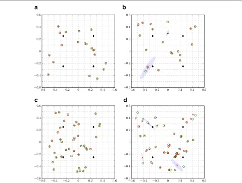
Another set of comparisons forN = 20 agents is pre-sented in Fig. 5b, where scenarios with 6 and 8 IDs are represented. Compared with the results shown in Fig.5a, increased variance is observed in the results, which leads to less steady average localization performance. Neverthe-less, it can be observed that the relaxed JLTAP algorithm still outperforms the optimal JLTAP algorithm, mainly because of the imposed run-time constraint of 5 days and the numerical challenges associated with the opti-mal JLTAP formulation. Exemplary localization results for two of the four tested configurations are presented in Fig. 6, where the actual agent positions are shown as green circles, the average position estimates are shown as red crosses, the anchor node positions are indicated by black diamonds, and the 1-standard-deviation regions are visualized as blue ellipses. The configurations shown
in Fig. 6a,b each contains 20 agents using 6 IDs. The average localization accuracies in terms of the RMSE are 2.0312 × 10⁻³and 1.1022 × 10⁻², respectively. Mean-while, the configurations shown in Fig.6c,deach contains 40 agents using 8 IDs. The average localization accuracies in terms of the RMSE are 1.9561 × 10⁻²and 4.4269× 10⁻², respectively. Results with somewhat high standard deviations (blue ellipses) occur mainly at the border of the environment, where the average connectivity is lower and localization is consequently more difficult.
It should be noted that the results discussed above are subject to two important effects with opposing complexity trends:
• With increasing connectivity, the number of measurements rises and the TAs consequently increase, resulting in a more complex optimization problem in the sense of greater numbers of constraints and variables.
• With increasing connectivity, measurements exists for more and more pairs of agents. Consequently, for R→ ∞, the effect of erroneously summed squared residual terms for pairs of agents without currently
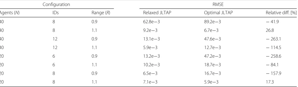
Table 3Exemplary values of the performance metric from Fig.5and their relative differences
Configuration RMSE
Agents (N) IDs Range (R) Relaxed JLTAP Optimal JLTAP Relative diff. [%]
40 8 0.9 62.8e−3 89.2e−3 −41.9
40 8 1.1 9.2e−3 6.7e−3 26.8
40 12 0.9 13.1e−3 47.6e−3 −263.1
40 12 1.1 5.9e−3 12.7e−3 −114.5
20 6 0.9 13.2e−3 47.2e−3 −258.6
20 6 1.1 10.2e−3 18.7e−3 −84.1
20 8 0.9 6.5e−3 16.7e−3 −157.9
a
b
c
d
Fig. 6All plots visualize average localization results (red crosses) and their 1-standard-deviation ellipses (blue ellipses) calculated over 100 simulations, in which the positions were held fixed and only the measurement noise was varied among the different simulations. The actual positions of the agents are shown by green circles, and the positions of the anchor nodes are indicated by black diamonds.aandbvisualize the statistics for two different random agent placements, each withN = 20 agents and 6 IDs. Likewise,canddvisualize the statistics for two different random agent placements, each withN = 40 agents and 8 IDs
hypothesized measurements is vanishing (cf. Item 13). This also limits the search space forqijasqij−−−→R→∞ 1.
5.4.2 Influence of measurement noise
Additional simulations were performed to analyze the robustness of the proposed relaxed JLTAP method with respect to measurement noise, and the results are pre-sented in Fig.7 for different sensing radii R. The figure shows that the localization error (RMSE) increases lin-early with the standard deviation of the measurement noise. Consequently, the relaxed JLTAP algorithm exhibits reasonable robustness with respect to measurement noise.
5.4.3 Run-time performance
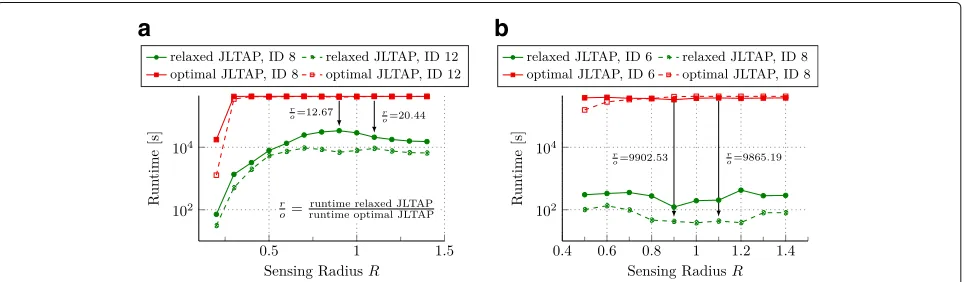
Run-time comparisons for both algorithms with the pre-viously described agent configurations are presented in
Fig.8. In both panels of the figure, the optimal JLTAP algo-rithm already reaches its maximal run-time constraint of 5 days for the moderate connectivity that results from a sensing radius ofR = 0.5. By contrast, the run time of the relaxed JLTAP algorithm varies, particularly in Fig.8a, which presents results from simulations withN = 40 agents. The drastic increase in run time for both algo-rithms is mainly due to the increased connectivity and the corresponding increase in combinatorial complexity (see also Section5.4.1first bullet).
6 Conclusions
a
b
Fig. 7Localization performance of the relaxed JLTAP algorithm with varying levels of measurement noise foraN = 40 agents with 12 IDs and
bN = 20 agents with 6 IDs
sensing agents. These application cases are relevant to novel and existing challenges arising, e.g., in the pas-sive localization of traffic participants, flying objects, or shooters and the surveying of resource-rich subterranean cavities (cf. Section1).
We have shown that the problem corresponding to the former application case is a special case of that corre-sponding to the latter. In the context of this problem, i.e., the problem of the joint localization of wireless agents and resolution of ambiguities in ranging measurements (the JLTAP), a detailed and thorough derivation and anal-ysis of the underlying graph-theoretical problem has been presented to serve as the basis for solving the problems arising in both application cases. Utilizing this description and the corresponding optimization problem formulation, we have derived and presented an MMSE-optimal JLTAP algorithm, and we have proven itsN P-hardness. More-over, to mitigate the exponential worst-case complexity of the optimal algorithm, we have derived a sub-optimal JLTAP algorithm through relaxations and approximations. In contrast to the existing literature on MSL in particu-lar, both formulations are capable of reflecting the likely
scenario in which sources or agents are not always in range of stations or beacons. Consequently, the presented algorithms not only are suitable for a broader variety of applications—such as those mentioned above—but also yield efficient solutions for a less restrictive set of scenar-ios corresponding to the existing application cases.
In the presented numerical evaluations, we have shown that the proposed sub-optimal algorithm offers signifi-cant gains in localization performance of up to 260% and reductions in run time by a factor of up to 9902. Con-sequently, efficient localization can be achieved, which is particularly important when many agents need to be localized.
6.1 Outlook
Because this work has focused on the more general prob-lem corresponding to Application Case 2 (cf. Section2), in our future work, we intend to analyze the proposed algorithms in direct comparison with existing MSL algo-rithms. We will also adapt the system model for different types of measurements, such as time-of-arrival (TOA) measurements6andpassive TOAmeasurements7.
a
b
Nomenclature
S Set of all serial numbers (SNs) used by the agents
Sa Set of all serial numbers (SNs) used
by the anchor nodes
I Set of all transmit IDs used by the agents
S(IJ) Set of agents that use IDIJ agenti Agent with the unique SN i
di,j Actual distance between agentsi
andj
dj→i Random variable (RV) denoting the
distance measured by agenti based on a signal from agentj
MIJ→i Tuple of measurements recorded
by agenti, e.g., MIJ→i=
. . .,mkIJ→i,. . .
, where k denotes the k th agent using IDIJ mkIJ→i Measurement (realization of the
corresponding RV) at agenti w.r.t. thek th agent usingIJ
Cekij Set of edges that arecopies of edge ekij
Pij Set of edges parallel to edge(i,j)
Shorthand version ofsuch that for sets; e.g.,∀x∈Rn x ≤1 defines then-dimensional unit ball around0
WA(e) Weight of edgee in the
corresponding ambiguity graph σij Standard deviation of the noise in
measurements between agentsi andj
σpi Standard deviation of the noise in the initial positions of the agents as used in the solver initialization pi,pˆi Actual and estimated Cartesian
positions of agenti
P Matrix of all agents’ Cartesian positions
ρ Vectorized form ofP
R Sensing, i.e., communication radius of the agents
[z]i i th component for vectorz
[pi]x, [pi]y X and Y coordinates of position
vectorpi
Endnotes
1Henceforth, the wireless sensor motes are also denoted
as agents.
2In addition, a shell that is sufficiently robust to
with-stand pressure levels of up to 6MPais required [30].
3The general principles and methods introduced in this
work can also be easily extended to other measurement models, such as those assuming multiplicative noise.
4The authors of [1] showed that it can take up to 48h for
an agent to pass through the environment.
5Here, we consider only strictly parallel edges; i.e.,
anti-parallel edges are disregarded.
6E.g., for the case in which the sources or agents are
actively sending their signals, whereas the stations or beacons are passive (listening only).
7In this case, the stations or beacons are sending signals,
whereas the sources or agents are passive, in the sense that they simply reflect these signals. The time of flight between the transmission of a pulse and the reception of a reflection is then measured.
Appendix 1: NP-hardness proof
The N P-hardness proof presented here makes use of a reduction from theperfect matching with conflict pair
con-straints (PMPC)problem, which is known to be strongly
N P-hard [31,32]. The corresponding decision problem is briefly described in the following.
Definition 2(Perfect matching with conflict pair
con-straints (PMPC) problem[31,32])
• The input: An undirected graphG = (V,E)and an undirected graphG¯ = (E,E¯), where each of the|E| vertices ofG¯belongs uniquely to one edgee∈EinG.
• The existence of an edge¯e∈ ¯Eimplies that the two adjacent vertices (edges ofG) cannot both appear simultaneously in the perfect matching (PM) ofG.
• The question: Does a PM inGexist such that adjacent vertices inG¯do not both belong to the PM?
To provide a concise proof, the following brief graph-theoretical summary of the problem defined in Definition1is used.
Definition 3(Graph-theoretical decision problem for-mulation of the JLTAP)
• The input: A(n) (un)directed graphG = (V,E)and several edge sets that belong uniquely to the following two categories (cf. Section3.1):
1. E=1=
iE=i1, 2. E≤1=iE≤i1,
• The question: Does a subsetE∗⊆Eexist such that exactly one edge from each non-empty setE=i1 appears inE∗and at most one edge from eachE≤i1 appears inE∗?
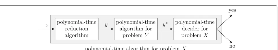
The N P-hardness proof is based on a Karp reduc-tion, the principle of which (proof by contradiction) is depicted in Fig.9. To complete the proof, we will define a time reduction algorithm and a polynomial-time decider. Subsequently, the correctness proof for the decider will be briefly outlined.
Definition 4(Polynomial-time reduction (PTR) algo-rithm) The PTR algorithm transforms an instance x of the PMPC problem into an instance y of the JLTAP decision problem by means of the following steps:
• The input: An instance x, i.e., two undirected graphs Gx = (Vx,Ex)andG¯x = (Ex,E¯x).
• The output: An instance y, i.e., an undirected graph G = (V,E)and several setsE=i1,i=1,. . .,n, and Ej
≤1,j=1,. . .,m.
• The transformation:
1. SetE:= ∅andV:=Vx.
2. For each vertexvi∈Vx, create a new setE=i1with all edges incident onvi.
3. For all edgese¯ij=(ei,ej)∈Ex×Ex, create a set
Eij
≤1= {ei,ej}.
Definition 5(Polynomial-time decider (PTD)) The PTD takes the output of the imaginary polynomial-time solver for the JLTAP decision problem and decides whether the answer to the problem instance x is yes or no.
• The input: The solutionE∗and the problem instance y corresponding toG=(V,E)and the sets{Ei
=1}i and{E≤j1}j.
• Return yes iff exactly one edge from each setE=i1and at most one edge from each setE≤j1are inE∗. Proof Sketch 1(Sketch of the Decider Correctness Proof )
To prove the correctness of the decision algorithm, the equivalence of the following two statements must be shown: A PM exists in the PMPC instance given byGand
¯
G. ⇔The solution set E∗is such that exactly one edge from each setE=i1and at most one edge from each setE≤i1 appear inE∗.
To see that this is the case, note that the existence of a PM in the PMPC instance means that there exists a set M⊆ Esuch that every vertex inGis incident on exactly one edge in the matchingM[33] and that for each con-flict pair in G¯, both edges do not appear simultaneously in the matching M. Mathematically, we can write this statement as
∃M⊆E such that |I(vi)∩M| = 1,∀vi∈V
()
and|A(e)∩M| = 0,∀e∈M ()
, (9)
whereI(v)denotes the set of edges incident on vertexv
andA(e)denotes the set of vertices in the conflict graph that are adjacent to vertexe. Recall that by the definition of the conflict graph (cf. Definition2), the vertices of the conflict graph are edges ofG.
The outline of the correctness proof given below shows that the two constraints()and() are inherently ful-filled by the definition of the reduction algorithm (cf. Definition4).
() By definition, the set of edges incident on vertexviis
given byE=i1, i.e.,I(vi)=E=i1. In addition, the
constraint|I(vi)∩M| =1means that exactly one of
these incident edges must be inM.
() Note thatA(e)denotes the set of edges that are in conflict with edgee and that these conflicts—with respect toe—are represented by|A(e)|sets of the formE≤i1= {e,ek}, whereek ∈A(e). The set
comprising these|A(e)|sets is henceforth denoted by E≤1(e). Consequently,A(e)can be written as follows:
A(e)= E∈E≤1(e)
E\e. (10)
Likewise, for constraint(), we have the following:
()⇔M∩
E∈E≤1(e)
E=∅, ife∈/M
e, otherwise ,∀e∈E.
(11)
Thus, its clear that()is equivalent to the
requirement that at most one edge from each setE≤i1 must be inE∗.
Appendix 2: Non-convexity of the relaxed JLTAP withqijequality constraint
In this section, the general non-convexity of the relaxed JLTAP objective function and, thus, of the relaxed JLTAP optimization problem is shown. Without loss of general-ity, the following summand of the objective function is considered for simplicity:
Hessian of (12) is partitioned into decision variablesxand positionsρ=
Let d be the shorthand notation for
d(ρ) = pi − pj 2 =
&
(x)2+(y)2, with
x = [pi]x − [pj]x,y = [pi]y − [pj]y. Then, the
partial derivatives can be written as follows:
∇2
By considering the Schur complement [34], it can be found that the Hessian off(·)is positive semi-definite, i.e., H(f)0, if and only if the following three conditions are whereAgdenotes the generalized inverse ofA.
Therewith, we form the following theorem regarding the non-convexity of (12):
Theorem 1The relaxed JLTAP objective as described in
Section4but with binding q := qij = kxkijas given in
(12)is non-convex for the relevant case of q>0.
ProofUsing Propositions 1 and 2, it holds regarding
Eqs. (15a) and (15b)
h≤0⇔ ∇ρρ2 f 0 and (16)
h≤0⇒=0. (17)
However, using Proposition4, it holds regarding (15c)
h≤0⇒S0, (18)
thus violating (15c) if (15a) is satisfied.
RemarkMoreover, the constraint h= ˜wx−d2≤0is non-convex.
Proposition 1∇ρρ2 f is positive semi-definitive, i.e.,
∇2
ρρf 0iff h≤0⇔d2≥ ˜wx.
ProofFrom straightforward calculations, we find that
∇2
ρρf has non-zero eigenvalues:
λ1
ProofAs the generalized inverse of∇ρρ2 f is given by
Proposition 3 Schur matrixSis given by:
Proposition 4Schur matrixSis negative semi-definite for h≤0.
ProofUsing the fact that a matrix Mis negative
semi-definite iffzM z≤0 for allz∈Rn,z=0, we obtain with Proposition 3 for the corresponding term of the Schur matrix:
After several algebraic steps, we find that the inner bracket is non-positive wheneverq >0 andh≤0. Con-sequently, we have for the relevant caseq >0:zS z≤ 0 ifh≤0.
Appendix 3: Similarities between the gradients of (5a) and (7a)
In this section, we analyze the similarities between the gradients of (5a), which is rewritten as
h(x,ρ)=(w+)x−d(ρ)2, (31)
and (7a), which is rewritten as
g(x,ρ)=(w+)◦2x−d(ρ)2
2
, (32)
where (x)◦2 denotes the Hadamard exponential, i.e., the element-wise exponential of the vector x; w =
The partial derivatives of (31) are given by
∇xh(x,ρ)=2
w∈x−d·w∈, (33) ∇ρh(x,ρ)= −2w∈x−d· ∇ρd, (34) wherew∈=w+andd=d(ρ).
Similarly, the following expressions hold for (32):
∇xg(x,ρ)=2 neously vanishing with respect tox(cf. Item 1) andρ(cf. Item 2) if and only if
Consequently, only the relaxation on the domain of x
(cf. (7b)) leads to different extrema of the two associated optimization problems.
Abbreviations
ID: Identification sequence; JLTAP: Joint localization and transmit ambiguity resolution problem; MSL: Multiple source localization; MINLP: Mixed-integer nonlinear programming; MMSE: Minimum mean square error; ML: Maximum likelihood; RMSE: Root mean square error SN: Serial number; TA: Transmit ambiguity; TOA: Time-of-arrival
Acknowledgements
We gratefully acknowledge the computational resources provided by the RWTH Compute Cluster from RWTH Aachen University under project RWTH0118.
Funding
This project has received funding from the European Union’s Horizon 2020 research and innovation program under grant agreement No. 665347.
Authors’ contributions
Competing interests
The authors declare that they have no competing interests.
Publisher’s Note
Springer Nature remains neutral with regard to jurisdictional claims in published maps and institutional affiliations.
Received: 31 October 2017 Accepted: 19 April 2018
References
1. E Talnishnikh, J van Pol, HJ Wörtche, inIntelligent Environmental Sensing. Smart Sensors, Measurement and Instrumentation, vol.13, ed. by H Leung, S Chandra Mukhopadhyay. Micro motes: a highly penetrating probe for inaccessible environments (Springer, Cham, 2015), pp. 33–49 2. Phoenix Project: EU Horizon 2020 FET-Open Project.http://www.
phoenix-project.euandhttp://cordis.europa.eu/project/rcn/196968_en. html. Accessed 31 Oct 2017
3. CM Istchenko, ID Gates, Well/wormhole model of cold heavy-oil production with sand. Soc. Petroleum Eng. J. 260–269 (2014).https://doi. org/10.2118/150633-PA
4. S Bhattacharjee, Oil sands: a bridge between conventional petroleum and a sustainable energy future. http://www.oilsands.ualberta.ca/wqm/wp-content/uploads/2010/09/Basu_BookChapter_Subir_Bhattacharjee_ June2010.pdf. Accessed 15 May 2017
5. A Hales, G Quarini, G Hilton, L Jones, E Lucas, D McBryde, X Yun, The effect of salinity and temperature on electromagnetic wave attenuation in brine. Int. J. Refrig.51, 161–168 (2015).https://doi.org/10.1016/j.ijrefrig. 2014.11.013
6. H Shen, Z Ding, S Dasgupta, C Zhao, Multiple source localization in wireless sensor networks based on time of arrival measurement. IEEE Trans. Signal Process.62(8), 1938–1949 (2014).https://doi.org/10.1109/ TSP.2014.2304433
7. S Venkateswaran, U Madhow, Localizing multiple events using times of arrival: a parallelized, hierarchical approach to the association problem. IEEE Trans. Signal Process.60(10), 5464–5477 (2012).https://doi.org/10. 1109/TSP.2012.2205919
8. Y Lee, TS Wada, BH Juang, in2010 IEEE International Conference on Acoustics, Speech and Signal Processing. Multiple acoustic source localization based on multiple hypotheses testing using particle approach, (2010), pp. 2722–2725.https://doi.org/10.1109/ICASSP.2010. 5496229
9. E Duisterwinkel, L Demi, G Dubbelman, E Talnishnikh, HJ Wörtche, JW Bergmans, inProc. Meetings Acoust.Environment mapping and localization with an uncontrolled swarm of ultrasound sensor motes, vol. 20 (Acoustical Society of America, San Francisco, 2014) 10. S Schlupkothen, G Ascheid, in2015 14th Annual Mediterranean Ad Hoc
Networking Workshop (MED-HOC-NET) (Med-Hoc-Net’15). Localization of wireless sensor networks with concurrently used identification sequences, (Vilamoura, 2015), pp. 1–7.https://doi.org/10.1109/ MedHocNet.2015.7173166
11. S Schlupkothen, G Ascheid, in2016 IEEE International Conference on Wireless for Space and Extreme Environments (WiSEE) (WiSEE’16). Joint localization and transmit-ambiguity resolution for ultra-low energy wireless sensors (IEEE, Aachen, 2016)
12. S Schlupkothen, B Prasse, G Ascheid, in2016 Mediterranean Ad Hoc Networking Workshop (Med-Hoc-Net). A dynamic programming algorithm for resolving transmit-ambiguities in the localization of wsn (IEEE, Vilanova i la Geltru, 2016), pp. 1–8.https://doi.org/10.1109/MedHocNet. 2016.7528420
13. EHA Duisterwinkel, G Dubbelman, L Demi, E Talnishnikh, JWM Bergmans, HJ Wörtche, in2016 IEEE Symposium Series on Computational Intelligence (SSCI). Mapping swarms of resource-limited sensor motes: solely using distance measurements and non-unique identifiers (IEEE, Athens, 2016), pp. 1–8.https://doi.org/10.1109/SSCI.2016.7849992
14. CA Floudas, PM Pardalos,Encyclopedia of optimization. Encyclopedia of optimization. (Springer, Secaucus, 2008)
15. J Aspnes, D Goldenberg, YR Yang, inAlgorithmic Aspects of Wireless Sensor Networks, ed. by SE Nikoletseas, JDP Rolim. On the computational complexity of sensor network localization (Springer, Berlin, 2004), pp. 32–44
16. P Biswas, Y Ye, inInformation Processing in Sensor Networks, 2004. IPSN 2004. Third International Symposium On. Semidefinite programming for ad hoc wireless sensor network localization (ACM, New York, 2004), pp. 46–54.https://doi.org/10.1109/IPSN.2004.1307322 17. AM-C So, Y Ye, inProceedings of the Sixteenth Annual ACM-SIAM
Symposium on Discrete Algorithms (SODA), 2005. Theory of semidefinite programming for sensor network localization (Society for Industrial and Applied Mathematics, Philadelphia, 2005), pp. 405–414
18. Z Wang, S Zheng, S Boyd, Y Ye, Further relaxations of the sdp approach to sensor network localization. Technical report (2006)
19. P Biswas, T-C Lian, T-C Wang, Y Ye, Semidefinite programming based algorithms for sensor network localization. ACM Trans. Sen. Netw.2(2), 188–220 (2006).https://doi.org/10.1145/1149283.1149286
20. P Biswas, T-C Liang, K-C Toh, Y Ye, T-C Wang, Semidefinite programming approaches for sensor network localization with noisy distance measurements. IEEE Transactions on Automation Science and Engineering.3(4), 360–371 (2006).https://doi.org/10.1109/TASE.2006. 877401
21. P Tseng, Second-order cone programming relaxation of sensor network localization. SIAM J. Optimization.18(1), 156–185 (2007).https://doi.org/ 10.1137/050640308
22. KWK Lui, WK Ma, HC So, FKW Chan, Semi-definite programming algorithms for sensor network node localization with uncertainties in anchor positions and/or propagation speed. IEEE Trans. Signal Process.
57(2), 752–763 (2009).https://doi.org/10.1109/TSP.2008.2007916 23. FKW Chan, HC So, Efficient weighted multidimensional scaling for
wireless sensor network localization. IEEE Trans. Signal Process.57(11), 4548–4553 (2009).https://doi.org/10.1109/TSP.2009.2024869 24. L Nguyen, S Kim, B Shim, in2016 Information Theory and Applications
Workshop (ITA). Localization in internet of things network: matrix completion approach (IEEE, La Jolla, 2016), pp. 1–4.https://doi.org/10. 1109/ITA.2016.7888154
25. GC Calafiore, L Carlone, M Wei, in18th Mediterranean Conference on Control Automation (MED), 2010. Position estimation from relative distance measurements in multi-agents formations (IEEE, Marrakech, 2010), pp. 148–153.https://doi.org/10.1109/MED.2010.5547601 26. BD Anderson, PN Belhumeur, T Eren, DK Goldenberg, AS Morse, W
Whiteley, YR Yang, Graphical properties of easily localizable sensor networks. Wirel. Netw.15(2), 177–191 (2009).https://doi.org/10.1007/ s11276-007-0034-9
27. J Aspnes, T Eren, DK Goldenberg, AS Morse, W Whiteley, YR Yang, BDO Anderson, PN Belhumeur, A theory of network localization. IEEE Transactions on Mobile Computing.5(12), 1663–1678 (2006).https://doi. org/10.1109/TMC.2006.174
28. S Schlupkothen, G Dartmann, G Ascheid, A novel low-complexity numerical localization method for dynamic wireless sensor networks. Signal Process. IEEE Trans.PP(99), 1–1 (2015).https://doi.org/10.1109/TSP. 2015.2422685
29. M Tawarmalani, NV Sahinidis, A polyhedral branch-and-cut approach to global optimization. Math. Program.103, 225–249 (2005)
30. MB Dusseault, CHOPS—Cold Heavy Oil Production with Sand in the Canadian heavy oil industry (2004).https://open.alberta.ca/dataset/ 2815953. Accessed 31 Oct 2017
31. T Öncan, R Zhang, AP Punnen, The minimum cost perfect matching problem with conflict pair constraints. Comput. Oper. Res.40(4), 920–930 (2013)
32. A Darmann, U Pferschy, J Schauer, GJ Woeginger, Paths, trees and matchings under disjunctive constraints. Discrete Appl. Math.159(16), 1726–1735 (2011). 8th Cologne/Twente Workshop on Graphs and Combinatorial Optimization (CTW 2009)
33. EW Weisstein, Perfect matching. From MathWorld—A Wolfram Web Resource (2016).http://mathworld.wolfram.com/PerfectMatching.html. Last visited on 08/30/2016