R E S E A R C H
Open Access
Design of robust high-order
superdirectivity for circular arrays with sensor
gain and phase errors
Min Wang
1*, Xiaochuan Ma
2, Ping Yang
1, Chengpeng Hao
2, Xiujuan Feng
1and Yue Zhang
1Abstract
Though the high-order superdirectivity theory proposed in recent years is attractive, it is hard to implement in practice due to its poor robustness to small random array errors. Hence, in this paper, we present two robust designs of high-order superdirectivity for circular arrays with gain and phase errors. Firstly, we study on the sensitivity function of the high-order superdirectivity and give an alternative solution for a robust superdirective beamformer based on sensitivity function constraint. This method could achieve an arbitrary compromise between directivity and robustness, so it is more flexible and applicable than the existing higher-order truncation method. Although it does not improve on computational complexity or performance with respect to the second-order cone programming obviously, it could lay the foundation for the following robust design method. Then, considering the fact that different eigenbeams correspond to different eigenvalues, we study the method of diagonal loading with variable factors in detail, and further improve the performance of the former sensitivity function constrained method by loading variable factors to different eigenbeams, which results in better performance and greater flexibility in making a compromise. We also show that this proposed loading variable factors method can achieve an equivalent result to the higher-order truncation method by setting proper factors. Simulation results demonstrate the robustness and effectiveness of the above two methods, especially the performance improvement of the loading variable factors method.
Keywords: High-order superdirectivity, Circular arrays, Array errors, Sensitivity function constraint, Diagonal loading, Loading variable factors
1 Introduction
Beamforming, which is a well-known approach to detect and enhance the desired signal while suppressing noise and interference with a sensor array, has been widely used in many applications [1, 2]. Among the performance mea-sures of a beamfomer, directivity describes the ability to suppress noise from all directions without affecting the desired signal from one principal direction.
As an optimal design in terms of directivity, superdirec-tivity [3–5] has attracted tremendous research in different disciplines such as radar [6, 7], sonar [8–12], audio engi-neering [13–16], and wireless communication [17, 18], etc. It is said that a superdirective array with relatively
*Correspondence: [email protected]
1Division of Mechanics and Acoustics, National Institute of Metrology, 100029 Beijing, China
Full list of author information is available at the end of the article
small size can provide much higher directivity than a con-ventional array does. In [19] and [20], it was proved that the maximum directivity factor (DF) of anM-sensor lin-ear array can reachM2at its endfire direction. It was also proved that the maximum DF of a spherical array isN2 withNbeing the mode number [21].
Compared to the widely used uniform linear array, uni-form circular array (UCA) has more compact structure and could form uniform beams over 360◦azimuthal direc-tions. So the superdirectivity of UCA has also attracted considerable attention [8–12, 18]. In [8] and [10], modal beamforming theory was used to analyse the superdirec-tivity of UCA, but it is not accurate enough due to the inevitable errors caused by spatial sampling and series truncation. Ma recently established a new theory of high-order superdirectivity for UCA [11]. It is based on eigen-decomposition of the circulant noise covariance matrix
and can provide an analytical and closed-form superdi-rective solution. So it is more accurate and attractive than the modal theory. Then, Wang made some extensions to this high-order superdirectivity theory. He extended it to a general superdirectivity model suitable for arbitrary arrays based on Gram-Schmidt mode-beam decomposition and synthesis [22]. Later, he also provided the analytical opti-mal solutions for the high-order superdirectivity of circu-lar arrays mounted on a rigid sphere and an infinite rigid cylinder [23].
Although theoretical superdirectivity seems to be very attractive, it is hard to be applied in real-world systems [5, 16, 24]. This is mainly because superdirectivity is very sensitive to the unavoidable random errors of practical arrays, such as sensor gain and phase errors, sensor posi-tion perturbaposi-tions, mutual coupling between sensors, etc. Small deviations can severely degrade the performance of superdirectivity, which may be even worse than that of the conventional beamforming. Thus, robust design meth-ods are eagerly needed to implement superdirectivity in practice.
Diagonal loading method [25] is very useful to improve the robustness, but the problem is that it is not clear how to choose the optimal loading factor. Yan presented a robust supergain beamforming via second-order cone programming (SOCP) [9], and Zhou provided a new superdirective beamforming method to jointly improve array efficiency and robustness for HF circular arrays [18]. But neither of them has provided the robust design solu-tion for the attractive high-order superdirectivity theory. Ma advised to improve the robustness by truncating the sensitive higher-order eigenbeams, i.e., the higher-order truncation (HOT) method [11]. However, this method can only truncate the eigenbeams by a step of certain inte-gral order, so it is not flexible and may be limited in many applications. Wang modified the weighting vector and simplified the diagonal matrix of eigenvalues by virtue of the symmetry properties, then they gave the solution in constraints of both sensitivity function (SF) and side-lobe level by the SOCP [12]. But loading variable factors to different eigenbeams still needs deeper investigation. Wang also discussed the robust design methods for the general superdirectivity model [22] and for the high-order superdirectivity of circular arrays mounted on rigid baf-fles [23]. Both of them have only used the reduced-rank technique, which is the same with the above HOT method in principle.
In this paper, the robustness of each eigenbeam is inves-tigated in detail for the high-order superdirectivity theory of UCA. Taking SF as the robustness parameter, we firstly give an alternative solution to a constrained superdirective beamformer (CSB) by adding a constraint to SF accord-ing to the errors, which is denoted as the CSB method. Although it does not make obvious improvements on
computational complexity or performance with respect to SOCP, the CSB method could lay the foundation for a fur-ther robust design. Precisely, based on the CSB method and considering that different eigenbeams correspond to different eigenvalues, we present a new design of loading variable factors (LVF) to different eigenbeams, which is named as the LVF method and results in improved perfor-mance. It will also be shown that this LVF method could easily achieve an equivalent result to the existing HOT method by setting proper factors.
The remainder of this paper is organised as follows. Firstly, some theory basis of high-order superdirectiv-ity for UCA is given in Sections 2 and 3. Specifically, the theory of high-order superdirectivity is described in Section 2, and its robustness is discussed in Section 3. The interested readers are referred to [11, 12] for further details. Then, Section 4 presents the two robust design methods. The performances of the proposed methods are demonstrated by simulation results in Section 5. Finally, the conclusions are summarized in Section 6.
2 High-order superdirectivity theory
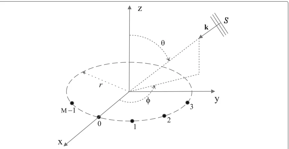
Consider an M-sensor UCA with radius r lying on the
xy-plane, as shown in Fig. 1. Assuming a unit magni-tude plane wave impinging from direction(φ,θ), where φ and θ are the azimuth and elevation angles,
respec-tively. The pressure received by the mth sensor at
(rcosφm,rsinφm, 0)can be expressed as
pm(φ,θ)=ejkrsinθcos(φm−φ), (1)
where k = 2π/λ is the wavenumber with λ being the
wavelength. Then, the array response vector of the UCA will be
Suppose the weighting vector and the present steer-ing direction besteer-ing denoted by w ∈ CM,1 and(φ0,θ0), respectively, the beam pattern (BP) will be
B(φ,θ)=wH(φ0,θ0)a(φ,θ). (3) It is known that solving the optimum weighting vector for the maximum DF is equivalent to maximizing the array gainGin an isotropic noise field [2, 11], i.e.,
wopt=arg max
w
wHa(φ0,θ0)2
wHρρρnw , (4)
where ρρρn is the normalized noise covariance matrix in an isotropic noise field.ρρρn is a circulant matrix and its mth eigenvalue and eigenvector are formulated asλm =
M−1
l=0 ρlejlφm andvm = √1M
Fig. 1Geometric model of anM-sensor uniform circular array
CM,1, respectively [26], whereρ
l = sinc(kdl) denotes
thelth element of the first row ofρρρnwithdlbeing the
sensor spacing between sensor 0 and sensor l[27]. It is easy to validate thatλm=λM−mandvm=v∗M−m.
By using the above property of the circulant symmet-ric matrixρρρn and expressingAm(φ,θ) = vHma(φ,θ), the
closed-form solutions of the optimal weighting vector, the maximum DF and the BP for superdirectivity can be obtained as [11, 12]
Thus, the maximum DF and the optimal BP for superdi-rectivity of a UCA are decomposed into the sum of the eigenbeams’ DFsDm and the sum of the eigenbeamsBm
(m = 0, 1,. . .,M/2), respectively. Based on these solu-tions, a complete theory of high-order superdirectivity for
UCA has been established. More details of this theory can be found in [11].
3 Analysis of robustness
Robustness, which measures the beamformer’s sensitivity to random errors, is a very crucial point in superdirec-tivity theory. So it is essential to discuss the robustness of the high-order superdirectivity before our methods are presented.
3.1 Robustness measurement
In [11], the eigenvalueλmhas been used as the robustness
parameter, but no detailed discussions are given. While Wang utilizes the SF to measure the robustness of high-order superdirectivity, since it is directly related to the sum of the variances of array errors and it could provide more information than eigenvalue [12]. We will also take the SF as the robustness measurement in the following discussions. Specifically, the larger the SF is, the poorer the robustness becomes.
The SF of the optimal superdirective beamformer is given by [12]
It is observed that the SF can also be decomposed into the sum of eigenbeams’ SFsTm, just as the maximum DF
the DFDmand the SFTmof each eigenbeam, which are
inversely proportional toλmandλ2m, respectively.
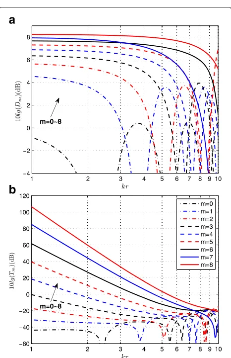
Figure 2 depicts the DFs Dm and the SFs Tm of
var-ious eigenbeams of a 16-sensor UCA both in decibels versus kr. It is seen that, for smaller kr, the higher the eigenbeam’s order is, the larger its DF is, yet the much larger its SF becomes. Askrincreases, both the DF and the SF decrease, the superdirective beamformer degrades to the conventional beamformer (CBF). Some related details of the DF and the SF of each eigenbeam are referred to [12].
3.2 An example
Providing an 8-sensor UCA withkr = 1 and(φ0,θ0) = (π/2,π/2), the actual gain gm and phase ϕm of themth
sensor are chosen according to
gm=1+
√
12σgβm, ϕm=
√
12σϕηm, (10)
a
b
Fig. 2Directivity factors and sensitivity functions of eigenbeams of a 16-sensor UCA both in decibels versuskr.aDirectivity factors 10 lg(Dm).bSensitivity functions 10 lg(Tm)
whereβmandηmare i.i.d. random variables in the uniform
distribution over [−0.5, 0.5],σg = 0.01 andσϕ = 1◦are
the standard deviations ofgmandϕm, respectively.
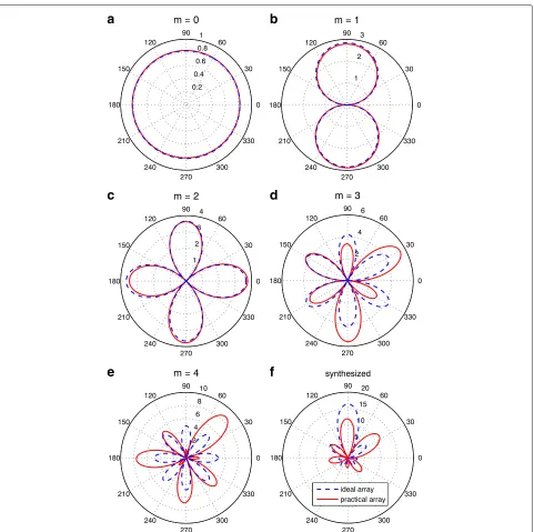
The eigenbeams and their synthesized BPs are shown in Fig. 3. For an ideal array without errors, the higher the eigenbeam’s order is, the larger its DF or gain is. While for this practical array with errors, some of its higher-order eigenbeams (m = 3, 4) are distorted obviously, which results in performance degradation of the synthesized BP as seen in Fig. 3f. This example validates the fact that, although the higher-order eigenbeam has higher gains, its robustness is very poor.
A useful way to improve the robustness is the HOT method presented in [11]. However, this method can only truncate the eigenbeams by a step of certain integral order, i.e. the adjustability between the SF and the DF is not flexible. So it may be limited in many applications.
4 Proposed algorithms
In this section, we first develop a method of design-ing the robust high-order superdirectivity based on the SF constraint. This design can be transformed into an extended diagonal loading problem, whose loading fac-tor is directly related to the SF constraint and can be solved by the existing numerical methods. Compared to the HOT method, it can achieve an arbitrary compromise between the superdirective beamformer and the conven-tional one. Then, although [12] has shown the concept of loading variable factors, it needs study in detail. So, based on the aforementioned high-order superdirectiv-ity theory, we investigate the method of loading variable factors to different eigenbeams, which could result in better performance and be more flexible to make a com-promise. Moreover, we will also see that an equivalent result to the HOT method could be achieved by setting proper factors.
4.1 The CSB method
Considering that the SF of a superdirective beamformer is undesirably high at low frequencies, we would add a con-straint on the SF to make the superdirective beamformer more robust. Denoting the maximum acceptable SF byδ0, the CSB will be
wcsb=arg min
w w
Hρρρnw,
subject to wHa(φ0,θ0)=1, Tsf= w2≤δ0. (11)
a
b
c
d
e
f
Fig. 3The 0th- to 4th-order eigenbeams and their synthesized beam patterns for an 8-sensor ideal UCA (blue dashed line) and an 8-sensor practical UCA (red solid line) withkr=1 and(φ0,θ0)=(π/2,π/2).am=0.bm=1.cm=2.dm=3.em=4.fSynthesized
The constraint factor δ0 is usually set by designers according to the practical array errors. This could be done by computer simulations or ad hoc experiments simply and efficiently. Specifically, the larger the array errors are, the smallerδ0should be, thus the more robust the CSB is, yet the smaller the DF is. It is noted that δ0 has a lower bound of 1/Mwhich corresponds to the CBF that is optimal in terms of robustness. In addition,δ0 should be smaller than or equal to the optimal superdirective beamformer’s SFTsfin (9), otherwise the added constraint
will be disabled. So the bound of the constraint factor is given by
1
M ≤δ0≤
aH(φ0,θ0)ρρρ−n2a(φ0,θ0)
aH(φ0,θ0)ρρρ−1
n a(φ0,θ0)
−2. (12)
Under the condition of (12), the SF constraintTsf =
w 2≤ δ0is enabled and the solution of (11) satisfies
wcsb=arg min
w w
Hρρρnw,
subject to wHa(φ0,θ0)=1, Tsf= w2=δ0. (13)
The solution of (13) can be obtained with the method of Lagrange multipliers [28], and is given by
wcsb= (ρρρn+γ
I)−1a(φ0,θ0)
aH(φ0,θ0) (ρρρ
n+γI)−1a(φ0,θ0)
, (14)
whereγ is a real-valued Lagrange multiplier withγ ≥ 0 and(ρρρn+γI) being positive definite, andI ∈ RM,M is a unit matrix. The factorγ can be calculated by the fol-lowing expression which linksγ to the preset constraint factorδ0directly,
It is seen from (14) that this design of the CSB belongs to the class of diagonal loading approaches essentially. The main difference between the CSB method and the tradi-tional loading sample matrix inversion (LSMI) method lies in that, it’s not clear how to choose the diagonal loading factor of the LSMI method, but the loading factor of our CSB method can be decided by the constraint factorδ0via Eq. (15).
Under the condition of (12), the middle term in
(15) is a monotonically decreasing function of γ
[28]. Denote this function by f(γ ), then f(0) =
aH(φ0,θ0)ρρρ−n2a(φ0,θ0)/aH(φ0,θ0)ρρρ−n1a(φ0,θ0)−2 and lim
γ→+∞f(γ ) = 1/Mjust correspond to the upper bound
and the lower bound ofδ0, respectively. Thus, Eq. (15) has a unique nonnegative solutionγˆ. Considering that (15) is a nonlinear equation, its solutionγˆ can be obtained effi-ciently by numerical methods such as a Newton’s iterative method.
Next, the upper bound ofγˆis worth discussing to avoid the trivial solution [28]. Sorting the eigenvalues{λm}Mm=−01
Substituting (16) into (15) and utilizing the relationship (ρρρn+ ˆγI)−1=U(+ ˆγI)−1UH, we will obtain
Representing the column vector UHa(φ0,θ0) by zand letting zm denote the mth element of z, (17) can be
By replacing λ¯m in the numerator and the
denomina-tor of (18) withλ¯M−1andλ0¯ , respectively, we can get an
Finally, summarizing the above design algorithm of the CSB as follows:
1) Perform eigen-decomposition on the normalized
noise covariance matrixρρρn.
2) Set a proper value for the constraint factorδ0 accord-ing to array errors. If (12) is satisfied, solve (18) forγˆ by a Newton’s iterative method under the condition of (20); otherwise, setγˆ =0.
3) Substitute theγˆobtained from Step 2 into (14) or
wcsb=
U(+γI)−1UHa(φ0,θ0)
aH(φ0,θ0)U(+γI)−1UHa(φ0,θ0) (21)
to calculate the desired weighting vector of the CSB.
It is noteworthy that both the SOCP and the CSB meth-ods require a complexity ofOM3[9, 28] and they can achieve the similar performance. But the CSB method could lay the foundation for the following LVF method and also facilitate the sequent comparison and analysis, so it is more suitable for the robust high-order superdirectiv-ity in this paper.
4.2 The LVF method
The above method achieves compromise between the DF and the SF by loading the same factorγˆ to all the eigen-values. Considering that the eigenvalues of high-order superdirectivity vary within a very wide range, e.g., the maximum eigenvalueλ0¯ =5.703 and the minimum eigen-valueλ4¯ =(4.025e−5)of an 8-sensor UCA withkr=1, we would expect that loading variable factors to differ-ent eigenvalues which correspond to differdiffer-ent eigenbeams will improve the above method to some extent.
Denoting the different loading factors byγˆm
M−1
m=0and using the original eigenvalues λm instead of the sorted
wlvf= These loading factors can be decided independently according to the eigenbeams’ robustness. Proper choosing of each loading factor will achieve a better compromise between the DF and the SF of a superdirective beam-former.
Further, from Eqs. (6), (7), and (9), we can see that for a very small eigenvalueλmwhich corresponds to a
high-order eigenbeam, its inverse 1/λm is infinitely large, so
that even small array errors may be greatly amplified. In this case, robustness is the main factor and we do not expect an accurate approximation of 1/λm, so a larger
loading factorγˆ2/λm is more proper thanγˆ. While for
a large eigenvalueλm, its eigenbeam is so robust against
array errors that there is no need to load any factor. And it can be easily seen thatλm+ ˆγ2/λm
with an increasing eigenvalue. Thus a loading factor which varies with its eigenvalue seems to be more reasonable than a fixed one.
Specifically, we propose to relate themth loading fac-tor γˆm with its corresponding eigenvalues λm and the
aforementioned solutionγˆ, i.e.,
ˆ
. Together with the modi-fied matrixGn =
ρρρn+ ˆγIin the above CSB method, the three matricesρρρn,Gn andRn have the same eigen-vectors and different eigenvalues λm,
two methods will be demonstrated in Section 5 by simu-lation results.
It should be noted that Eq. (23) is mainly taken as one example to show the potential improved performance of the LVF method. The analytical optimal solution for vari-able factorsγˆm
M−1
m=0still needs more investigation, and it would be one of our main future research tracks.
Before closing this section, we will show the relationship between this LVF method and the aforementioned HOT method. From (6) and (9), the DF and the SF of the mth-order eigenbeam with a variable loading factorγˆmcan be
respectively expressed as
Tmboth equal 0, which means themth-order eigenbeam
is not available, or i.e., truncated. The other isγˆm = 0,
thus the DFDˆmand the SFTˆmkeep unchanged with their
counterparts in the high-order superdirectivity theory, so that the mth-order eigenbeam will be reserved. In con-clusion, the result of the HOT method, which can also be implemented by settingγˆm =0 to the lower-order
eigen-beams andγˆm = +∞to the higher-order eigenbeams, is
contained in our LVF method.
5 Simulation results
In this section, some simulation results are presented to illustrate the performances of the proposed methods. Firstly, the design of the CSB is shown with several dif-ferent SF constraint factors. Then, the performances of the CSB method and the LVF method are compared by a design example. At last, the relationship between the LVF method and the HOT method is shown and discussed. Without loss of generality, the present steering direction is set as(φ0,θ0)=(π/2,π/2)in the following simulations.
5.1 Simulations of the CSB method
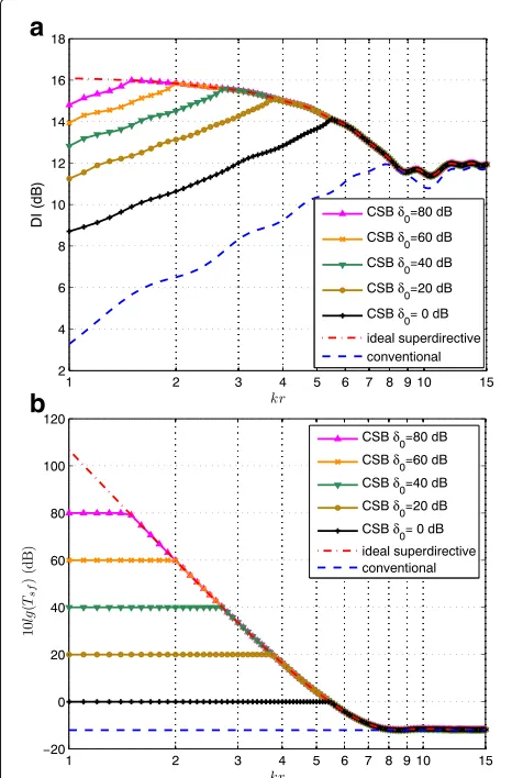
Consider a 16-sensor UCA withkrranging from 1 to 15, the SF constraint factorδ0is set as 80, 60, 40, 20, and 0 dB, respectively. The total DF (or its logarithmic form the directivity index (DI), which is defined as DI=10 lg(DF) (dB)) and SF of the CSB are depicted in Fig. 4. The con-ventional and ideal superdirective results are added for comparison, where the conventional result is obtained by using the weighting vector w = a(φ0,θ0)/M, and the ideal superdirective result is obtained by using the optimal weighting vector in (5). Some relevant conclusions can be made as follows.
It is shown from Fig. 4 that, for the ideal superdi-rective beamformer, its DF decreases and its SF drops more quickly as kr increases, it will finally degrade to the conventional beamformer since the normalized noise covariance matrixρρρntends to a unit matrix. These results have just validated the fact that superdirectivity can only be achieved for smallkr[13].
In Fig. 4b, the SF of the proposed CSB is seen to be constrained less than or equal to the SF constraint factor δ0, while the corresponding DF decreases to a certain extent, as shown in Fig. 4a. The smaller the
SF constraint factor δ0 is, the more robust the CSB
a
b
Fig. 4Total directivity index and sensitivity function of the CSB versus
krwith various constraint factors.aDirectivity index.bSensitivity function
It should be noted that, if (12) is satisfied, the constraint factorδ0is effective and equal to the SF of the CSB; but when δ0 is larger than the SF of superdirectivity as kr increases, it will be ineffective, then the CSB is equivalent to the superdirective beamformer, as shown in Fig. 4.
5.2 Comparisons of the CSB and LVF methods
To compare the performances of the CSB and LVF meth-ods, we setδ0 = 20 dB andM =12. The loading factors
ˆ
γ and { ˆγm}Mm=−01 are, respectively, computed by (18) and (23). The total DI (or DF in decibel) and SF are shown in Fig. 5.
It is seen from Fig. 5b that, for smallkr, the SF of the CSB is constrained to be δ0 while the SF of the LVF is variable and lower than δ0 at most points. Meanwhile, the DFs of the LVF and the CSB remain almost the same level, as shown in Fig. 5a. Askrincreases, both the CSB and LVF methods become the superdirective beamformer and tend to the conventional one finally. These results
a
b
Fig. 5Total directivity index (or directivity factor in decibel) and sensitivity function of the CSB and the LVF versuskrfor a 12-sensor UCA.aDirectivity index.bSensitivity function
show that the LVF method could achieve a more flexible compromise than the CSB method between superdirec-tivity and robustness. Moreover, the LVF method is some-what more robust for most smallkr.
Next, we add some random gain and phase errors to the 12-sensor array withkr = 1.5 according to (10) with σg =0.01 andσϕ =1◦, and examine the eigenbeams and
synthesized BPs of four cases (superdirectivity of the prac-tical array with errors, superdirectivity of the ideal array without errors, CSB design with array errors, and LVF design with array errors).
a
b
c
d
e
f
Fig. 6The 2nd- to 6th-order eigenbeams of four cases (practical array , ideal array, LVF design and CSB design) for a 12-sensor array withkr=1.5 in the presence of array gain and phase errors.am=2.bm=3.cm=4.dm=5.em=6.fMagnification of a portion ofe
seriously distorted due to their poor robustness, while these two eigenbeams of the CSB and LVF methods are significantly reduced, especially the LVF case. That is why the robustness could be improved by using the CSB and LVF methods.
Figure 7 depicts the total BPs of the four cases. Again, Fig. 7b is a magnification of a portion of Fig. 7a with the CBF for comparison. The superdirective BP of the practi-cal array with gain and phase errors (labelled as “practipracti-cal” in Fig. 7a), which is synthesized using all practical eigen-beams from order 0 to order 6, is shown to be extremely
a
b
Fig. 7Comparison of total beam patterns with gain and phase errors for a 12-sensor UCA,kr=1.5.aTotal beam patterns without including CBF.b
Magnification of a portion ofawith CBF
the CSB method. In addition, the BP of the LVF method is more symmetrical and its shape is closer to the ideal BP, which means that the LVF method is more robust to gain and phase errors than the CSB method.
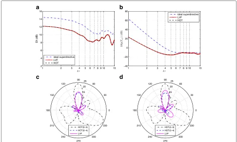
To compare the performance of the two methods fur-ther, we change the simulation conditions withM = 16, kr = 1.65 andδ0 = 30 dB. The levels of gain and phase errors keep unchanged. The simulation results of the total BPs are shown in Fig. 8. We can see that the performance of the BP of the LVF method outperforms that of the CSB method obviously. Although its mainlobe is some-what widened, the sidelobe level and the shape of the BP of the LVF method are much improved, while the BP of the CSB method is relatively poor in performance.
At last, comparing the results of Figs. 7b and 8a, we can find that the DF achieved by the LVF method is better than that of the CSB method in Fig. 8a, while it is somewhat worse in Fig. 7b. The main reason lies in that the BPs of
the two methods are distorted in varying degrees by array errors. In Fig. 7b, the SF constraint factorδ0is 20 dB, so both the BPs of the two methods are relatively less dis-torted. The DF of the LVF method is a little worse than that of the CSB method, but the LVF method is shown to be more robust. This is reasonable because the DF and the SF are a pair of tradeoffs theoretically. While in Fig. 8a, δ0is increased to 30 dB and the array errors play a main role in this case. The two BPs are distorted more seriously, especially the CSB method. So the DF of the LVF method is better because its BP is less affected by array errors than that of the CSB method.
5.3 The LVF method versus the HOT method
In the last simulation, we will illustrate the relationship between our LVF method and the existing HOT method.
Reconsider a 12-sensor UCA, and set the loading fac-tors γˆm as +∞ for m = 5, 6, 7, and 0 for the others,
b
a
respectively. Actually, this is equivalent to loading +∞ to the 5th- and 6th-order eigenbeams and loading 0 to the 0th- to 4th-order ones since λm = λM−m. On the
other hand, truncate the 5th- and 6th-order eigenbeams directly using the HOT method. The corresponding total DI (or DF in decibel) and SF are shown in Fig. 9a and b, respectively. It can be seen that both of the DFs and SFs of the two methods match well with each other. So our LVF method could obtain an equivalent result to the HOT method by properly setting 0 and+∞to the loading factors.
Then, under the condition of the aforementioned array
errors with kr = 1.5, we design the HOT method by
synthesizing the 0th- to 5th-order eigenbeams and the 0th- to 4th-order eigenbeams, respectively, and design
the LVF method by setting δ0 = 20 dB. The BPs of
the three cases are shown in Fig. 9c. It is seen that
the LVF method has the similar BP to the HOT(0∼4)
method. Although its mainlobe width is about 7◦broader than that of the HOT(0∼5) method, its sidelobe level (about −6.66 dB) is very much improved since the BP of the HOT(0∼5) method is severely distorted and use-less. Further, we increase the constraint factor of the
LVF method to δ0 = 23 dB in Fig. 9d. Compared with
the HOT(0∼4) method, the mainlobe width of the LVF
method is reduced by about 2.5◦, but its sidelobe level is increased by about 0.5 dB. Moreover, the LVF method is still much more robust than the HOT(0∼5) method. These results show the fact that the LVF method could adjust the compromise between directivity and robustness more flexibly.
Thus, our LVF method could fill the gap between differ-ent eigenbeams truncations of the HOT method, and it is more flexible to make a compromise and has the potential to provide better performance in the robust design of high-order superdirectivity.
6 Conclusions
In conclusion, we make a detailed study of the variable loading method for improving the robustness of high-order superdirectivity for circular arrays. Since higher-order eigenbeams are very sensitive to array gain and phase errors, the theoretical superdirectivity is hardly implemented in practice. To solve this problem, we present two robust design methods in this paper. Firstly, by adding a constraint to the SF, a more robust CSB is produced which can achieve a compromise between the superdirective beamformer and the conventional one, in terms of directivity and robustness. Further, a more flexi-ble LVF method is proposed by loading variaflexi-ble factors to
a
b
c
d
different eigenbeams, and it has better performance than the CSB method at most frequencies. We also prove that the LVF method contains the results of the existing HOT method and could outperform it. Simulation results have demonstrated that the robustness of high-order superdi-rectivity to gain and phase errors is obviously improved by the proposed methods. The effects of other factors on high-order superdirectivity, such as mutual coupling and array efficiency, still need more investigation, and it would be our another main future research track.
Acknowledgements
The authors would like to thank the anonymous reviewers for their insightful comments and suggestions, which helped improve the quality of this paper significantly.
Funding
This work was supported by the National Natural Science Foundation of China under Grants 51505453, 61471352 and 61571434.
Authors’ contributions
MW and XCM conceived the basic idea and designed the numerical simulations. MW and PY analyzed the simulation results. CPH analyzed derivation of equations and revised the manuscript. XJF and YZ checked the simulations and refined the whole manuscript. MW wrote and revised the manuscript. All authors read and approved the final manuscript.
Competing interests
The authors declare that they have no competing interests.
Author details
1Division of Mechanics and Acoustics, National Institute of Metrology, 100029 Beijing, China.2Institute of Acoustics, Chinese Academy of Sciences, 100190 Beijing, China.
Received: 16 August 2016 Accepted: 14 February 2017
References
1. H Krim, M Viberg, Two decades of array signal processing research: the parametric approach. IEEE Signal Proc. Mag.13, 67–94 (1996)
2. HL Van Trees,Optimum Array Processing: Part IV of Detection, Estimation, and
Modulation Theory. (Wiley, New York, 2002), pp. 59–71, 274–289, 439–443
3. EH Newman, JH Richmond, CH Walter, Superdirective receiving arrays. IEEE Trans. Antennas Propag.26(5), 629–635 (1978)
4. M Crocco, A Trucco, Design of robust superdirective arrays with a tunable tradeoff between directivity and frequency-invariance. IEEE Trans. Signal Process.59, 2169–2181 (2011)
5. A Trucco, M Crocco, Design of an optimum superdirective beamformer through generalized directivity maximization. IEEE Trans. Signal Process.
62, 6118–6129 (2014)
6. DP Scholnik, JO Coleman, inIEEE Radar Conf.Superdirectivity and SNR constraints in wideband array-pattern design (IEEE, Atlanta, 2001), pp. 181–186
7. ML Morris, MA Jensen, JW Wallace, Superdirectivity in MIMO systems. IEEE Trans. Antennas Propag.53(9), 2850–2857 (2005)
8. JB Franklin,Superdirective receiving arrays for underwater acoustics
application. (DREA Report No. CR/97/444, Defence Research
Establishment Atlantic, Dartmouth, Nova Scotia, 1997)
9. SF Yan, YL Ma, Robust supergain beamforming for circular array via second-order cone programming. Appl. Acoust. (Elsevier).66(9), 1018–1032 (2005)
10. YX Yang, W Jiang, YL Ma, inOCEANS 2007. Phased-mode circular multi-channel hydrophone with super directivity (IEEE, Vancouver, 2007), pp. 1–5
11. YL Ma, YX Yang, ZY He, KD Yang, C Sun, YM Wang, Theoretical and practical solutions for high-order superdirectivity of circular sensor arrays. IEEE Trans. Ind. Electron.60, 203–209 (2013)
12. Y Wang, YX Yang, YL Ma, ZY He, Robust high-order superdirectivity of circular sensor arrays. J. Acoust. Soc. Am.136(4), 1712–1724 (2014) 13. J Bitzer, KU Simmer, inMicrophone arrays: Signal Processing Techniques and
Applications. Superdirective microphone arrays (Springer-Verlag, New
York, 2001), pp. 19–38
14. TD Abhayapala, DB Ward, inIEEE International Conference On Acoustics,
Speech and Signal Processing (ICASSP). Theory and design of high order
sound field microphones using spherical microphone array (IEEE, Florida, 2002), pp. 1949–1952
15. TD Abhayapala, A Gupta, Spherical harmonic analysis of wavefields using multiple circular sensor arrays. IEEE Trans. Audio Speech Lang. Process.
18(6), 1655–1664 (2010)
16. S Doclo, M Moonen, Superdirective beamforming robust against microphone mismatch. IEEE Trans. Audio Speech Lang. Process.15(2), 617–631 (2007)
17. NW Bikhazi, MA Jensen, The relationship between antenna loss and superdirectivity in MIMO systems. IEEE Trans. Wirel. Commun.6(5), 1796–1802 (2007)
18. Q-C Zhou, HT Gao, HJ Zhang, F Wang, Robust superdirective beamforming for hf circular receive antenna arrays. Prog. Electromagn. Res.136, 665–679 (2013)
19. AI Uzkov, An approach to the problem of optimum directive antenna design. Compt. Rend. Acad. Sci. U.R.S.S.53, 35–38 (1946)
20. AT Parsons, Maximum directivity proof for three-dimensional arrays. J. Acoust. Soc. Am.82(1), 179–182 (1987)
21. JL Butler, SL Ehrlich, Superdirective spherical radiator. J. Acoust. Soc. Am.
61(6), 1427–1431 (1977)
22. Y Wang, YX Yang, ZY He, YN Han, YL Ma, A general superdirectivity model for arbitrary sensor arrays. EURASIP J. Adv. Signal Process.2015(1), 1–16 (2015)
23. Y Wang, YX Yang, YL Ma, ZY He, High-order superdirectivity of circular sensor arrays mounted on baffles. Acta Acust. united Ac.102(1), 80–93 (2016)
24. H Cox, RM Zeskind, T Kouij, Practical supergain. IEEE Trans. Acoust. Speech Signal Process.34(3), 393–398 (1986)
25. BD Carlson, Covariance matrix estimation errors and diagonal loading in adaptive arrays. IEEE Trans. Aero. Elec. Syst.24(3), 397–401 (1988) 26. RM Gray, Toeplitz and circulant matrices: a review. Found. Trends
Commun. Inf. Theory.2(3), 155–239 (2006)
27. BF Cron, CH Sherman, Spatial-correlation functions for various noise models. J. Acoust. Soc. Am.34(11), 1732–1736 (1962)
28. J Li, P Stoica, ZS Wang, Doubly constrained robust Capon beamformer. IEEE Trans. Signal Process.52(9), 2407–2423 (2004)
Submit your manuscript to a
journal and benefi t from:
7Convenient online submission
7 Rigorous peer review
7Immediate publication on acceptance
7 Open access: articles freely available online
7High visibility within the fi eld
7 Retaining the copyright to your article