R E S E A R C H
Open Access
MapReduce particle filtering with exact
resampling and deterministic runtime
Jeyarajan Thiyagalingam, Lykourgos Kekempanos and Simon Maskell
*Abstract
Particle filtering is a numerical Bayesian technique that has great potential for solving sequential estimation problems involving non-linear and non-Gaussian models. Since the estimation accuracy achieved by particle filters improves as the number of particles increases, it is natural to consider as many particles as possible. MapReduce is a generic programming model that makes it possible to scale a wide variety of algorithms to Big data. However, despite the application of particle filters across many domains, little attention has been devoted to implementing particle filters using MapReduce.
In this paper, we describe an implementation of a particle filter using MapReduce. We focus on a component that what would otherwise be a bottleneck to parallel execution, the resampling component. We devise a new
implementation of this component, which requires no approximations, hasO(N)spatial complexity and deterministic O(logN)2time complexity. Results demonstrate the utility of this new component and culminate in consideration of a particle filter with 224particles being distributed across 512 processor cores.
Keywords: MCMC methods, Particle filters, Big data sampling, MapReduce, Resampling
1 Introduction
Particle filters are a Bayesian Monte-Carlo method that provide a general framework for estimation in response to an incoming stream of data. The key idea is to rep-resent the probability density function (pdf ) of the state of a system using random samples (known as parti-cles). These samples are propagated across iterations in time in a way that capitalises on an application-specific non-linear, non-Gaussian space model. This state-space model describes both the dynamic evolution of the state and the relationship between the state and the measurements. The use of random samples to articu-late uncertainty means that particle filters can be applied to a variety of real-world problems without any need to approximate the models used. This is in contrast to alter-native techniques (e.g., the Extended Kalman filter; EKF) that approximate the models such that the uncertainty present can be approximated using a parametric probabil-ity densprobabil-ity (a multivariate Gaussian in the case of an EKF). The result is that a particle filter typically outperforms
*Correspondence: [email protected]
Department of Electrical Engineering and Electronics, University of Liverpool, Liverpool L69 3GJ, UK
such alternative techniques in scenarios involving pro-nounced departures from linear-Gaussian models. Such scenarios are widespread. This is arguably the reason why particle filters, since their inception [1], have been applied successfully in such a diverse range of contexts [2–5].
Particle filters have the appealing property that, as the number of samples increases, the ability of the samples to represent the pdf increases and the accuracy of estimates derived from the particles improves: an upper-bound on the variance of an estimate scales asON1[6]. It is there-fore natural to seek to use as many particles as possible. However, when the number of samples becomes very large, the samples will not physically fit within the mem-ory space of a single compute node. Big data platforms have been developed to address the generic problem of which this is a special case. These platforms work by iden-tifying abstractions of algorithms that make the potential for parallelism apparent. The platforms (and not the pro-grammer) are then able to exploit the available computa-tional resources to distribute the processing. One popular abstraction is MapReduce (which is described in more detail in Section 2.2). Various techniques have been devel-oped to distribute particle filters across multiple processor
cores (see Section 7 for the details), but MapReduce has not been used with particle filters extensively (that said, [7] and [8] are counter-examples we are aware of ).
The resampling component is a critical component of a particle filter and non-trivial to parallelise. As will be dis-cussed in more detail in Section 7, previous approaches to distributing the resampling step have focused on mod-ifying the resampling process with the aim of making it more amenable to distributed implementation. One notable exception exists [9]1 and ensures that the out-put from the distributed implementation is exactly that output from a single-processor implementation while also ensuring deterministic2data transfer and runtime. Such deterministic runtime is important in real-time applica-tions (which are widespread) where the output of the particle filter is used to feed the input of another pro-cess, which needs to receive that input within a specified latency.
In this paper, we present an improved parallel imple-mentation strategy for the resampling component, a MapReduce representation of the particle filter (including this resampling component) and instantiate the particle filter in the context of two Big data platforms. In doing so, this paper makes the following key contributions:
• We propose an improved implementation of an exact deterministic resampling algorithm that has better temporal complexity compared to the current state-of-the-art [9]. More specifically, the proposed version of the parallel algorithm has the complexity ofO(log2N)2compared to the original complexity
ofO(log2N)3.
• We provide two different MapReduce variants of our new algorithm that fit both with the in-memory processing and out-of-core processing models. These are the processing models used by Hadoop and Spark respectively.
• We perform detailed performance and scalability analysis of our new algorithm in comparison to both the pre-existing state-of-the-art [9] and an
implementation optimised for a single-processor core. We deliberately chose an application that stresses the resampling component of the particle filter such that our analysis relates to the worst-case performance.
The remainder of this paper is organised as follows: In Section 2, we provide a brief overview of Big data pro-cessing, and the MapReduce programming model. This is then followed by a detailed description of particle filtering in Section 3. In Section 4, we describe the fundamental building blocks that are used to construct the imple-mentations of the particle filtering algorithm, including, in Section 4.8.2, the new component of the resampling
algorithm. We then describe our MapReduce-based par-ticle filtering implementation in Section 5. We follow this section with an evaluation of our algorithms on key two MapReduce frameworks in Section 6. Section 7 highlights related work before Section 8 concludes.
2 Big data processing
The focus in this paper is on the problem of using large numbers of samples within a particle filter. Big data processing frameworks (e.g., Apache projects such as: Hadoop [10], Spark [11] and Storm [12]3) are designed for handling large amounts of data and can therefore be applied in this context4. We therefore focus in this paper on using such frameworks in conjunction with par-allel computational resources, such as clusters, to handle large volumes of data5. In this section, we discuss the use of such Big data frameworks in general and, in particu-lar, one of the programming models that underpins such frameworks, the MapReduce programming model.
2.1 Big data frameworks
An attractive approach for scaling the problem with data is to use Big data frameworks. More strictly, Big data frame-works go beyond the issue of data volume and address much wider issues covering augmented V’s of data, for instancevolume, velocity, variety, valueandveracity[13]. Big data framework-based solutions are process-centric: the programmer describes the algorithm in a way that enables the framework itself to understand (and attempt to exploit) the potential to distribute the data and process-ing6. The result of this delegation of the optimisation for speed to the framework is that, while many of today’s Big data frameworks can handle large volumes of data, none can match the runtime performance of conventional HPC systems [14].
There are a growing number of different programming models that are used to describe algorithms within Big data frameworks. These models include MapReduce [15], Stream Processing [11, 12, 16] and Query-based tech-niques [17, 18]. Here, we focus on one such programming model, MapReduce.
2.2 The MapReduce programming model
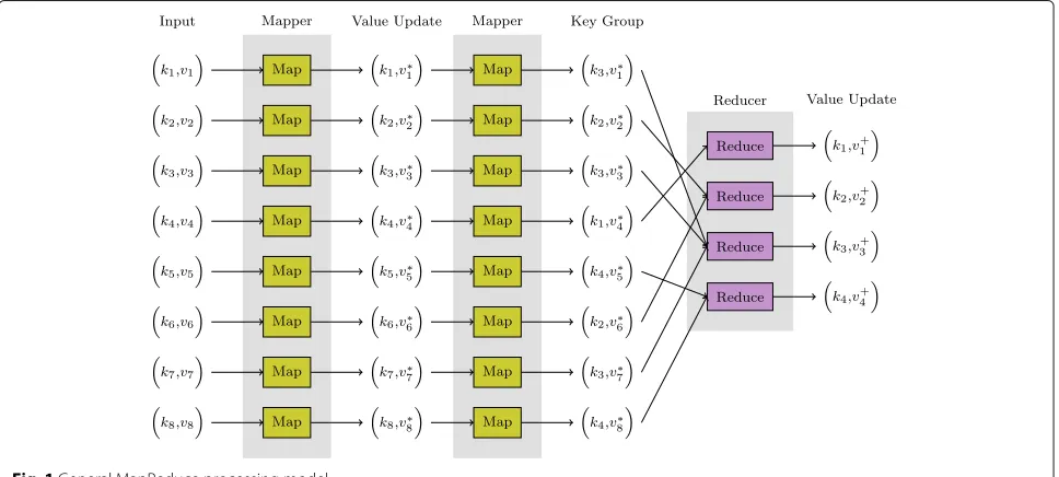
inherently parallel across all data and keys respectively7. To exemplify this, consider a dataset where each datum is a sentence in a Big document (e.g., Wikipedia). The problem of counting the total number of occurrences of each word in the document corpus can then be described as using the words as the key, a mapper that outputs a (non-zero) count of the number of times each word occurs in each sentence8and a reducer that calculates the sum of the counts. For each word, the reducer’s output is then the sum over all sentences of the counts per sen-tence. Another example is shown in Fig. 1 and illustrates the ability to pass (key, value) pairs into a mapper and thereby use the output of one mapper as the input into a second mapper.
Two key frameworks that support MapReduce, albeit in slightly different ways, are Hadoop and Spark. These are now considered in turn.
2.2.1 Hadoop
MapReduce is one of the two fundamental components of Hadoop. The other is the Hadoop Distributed File System (HDFS). HDFS enables multiple computers’ disks to be accessed in much the same way as if it were a single (Big) disk. In Hadoop, the mapper and reducer generate files which are stored in HDFS, such that Hadoop implements data movement entirely via the file system.
2.2.2 Spark
The Spark framework operates using a different princi-ple. First, at the Application Programming Interface (API) level, Spark provides a distributed data structure known as a Resilient Distributed Dataset (RDDs) [19]. MapRe-duce is then just one of a large number oftransformations
that (via a rich set of APIs) can be applied to RDDs. It is also important to realise that evaluations in Spark arelazilyexecuted. This means, unlike conventional pro-cessing engines (e.g., Hadoop), executions never actu-ally happen when transformations are defined. Instead, transformations are used to compose a data-flow graph and execution happens when forced throughactions(i.e., when necessary). This delayed evaluation enables the Spark framework to optimise (and plan) the execution9. The result is often significant improvements in runtime performance. Another important property of RDDs is that they can reside in the memory, disk or in combination. Indeed, although Spark can make use of HDFS, the data movements in Spark are primarily via memory. Again, this can result in significant improvements in runtime performance relative to Hadoop.
3 Particle filtering
We now provide a brief description of particle filtering. The reader unfamiliar with particle filtering is referred to [20]. Here, we aim to introduce notation and contextualise the discussion in the subsequent sections.
Let{x}k=1,2,..be the discrete-time Markov process rep-resenting the collection of states and {z}k=1,2,.. be the sequence of measurements.p(xk|xk−1)is the state transi-tion probability andp(zk|xk)is the likelihood. Recursive Bayesian filtering is the solution to the problem of using these models to process incoming data to obtain the posterior probability density function, p(xk|z1:k), where
z1:k = {zi,i= 1,. . .,k}is the sequence of measurements up to and including time k. p(xk|z1:k) is the sufficient statistic used to calculate, for example, estimates of the current state vector.
In a particle filter, the posterior is approximated using a set ofNrandom samples, where theith sample isxikand has a weight ofwik.
The weights are normalised such that Ni=1wik = 1. Estimates associated with the posterior at timekcan then be approximated as: lating the mean). As the number of samples increases, the approximation becomes increasingly accurate. In fact, the variance of the estimate in (1) can be shown to be upper-bounded by a quantity that is proportional toN1.
3.1 Sequential importance sampling
Importance sampling [21] is a technique for approximat-ing one pdf usapproximat-ing weighted samples from another pdf. A sequential importance sampler (SIS) involves applying importance sampling to the path10 through the state-space,x1:k. The samples up to timekare also assumed to be generated by extending the samples of the path up to timek−1. This enables the weights in SIS to be derived as [22]: generatexkand where
wi1∝ p the initial state and the initial distribution of samples (both atk=1).
Note that, when each measurement is received, SIS involves sampling particles fromqxk|xk−1,zk
and then updating their weights using (2).
3.2 Degeneracy problem
With the SIS algorithm, the variance of the importance weights can be proved to increase over time [22]11. Empir-ically, this results indegeneracy: all but one particle ends up having negligible normalised weights such that a single particle dominates the weighted average in (1). A way to quantify this effect is to calculate the effective sample size, Neff, introduced in [23] and estimated as follows:
Neff =
Neff dropping below a threshold,NT, indicates that esti-mates are likely to be inaccurate. The key to addressing this is to introduceresampling. The basic idea of resam-pling is to eliminate samples with low importance weights and replicate samples with larger weights12. While there are a number of variants of the resampling algorithm, they all consist of two core stages: calculating how many copies of each sample to generate and generating that number of copies of each sample. The different resam-pling variants differ in terms of how they calculate the number of copies to generate. We focus here onminimum variance resampling (also known as systematic resam-pling) which minimises the errors inevitably introduced by the resampling process (and is discussed in more detail in Section 4.6). The use of resampling with SIS is often known as the sampling importance resampling (SIR) fil-ter and has been at the heart of particle filfil-ters since their invention [1, 24, 25].
Algorithm 1 shows pseudocode for the SIR filter. Note that the algorithm is expressed in vector notation, such
Algorithm 1SIR Filter—Sequential (Vectorized) Version 1: FunctionsirFilter(p(x0),p(zκ|xκ),p(xκ|xκ−1),q(xκ|xκ−1,zκ))
2: p(x0): the initial prior
3: p(zκ|xκ): measurement model
4: p(xκ|xκ−1): dynamic model
5: q(xκ|xκ−1,zκ): proposal
6: Initialize the Particles
7: x0←drawSample(p(x0))
13: Calculate New Weights
14: w∗k←wk−1p(zqk(|xxkk|)xpk(−xk1,z|xkk)−1)
15: Normalise the Weights
16: wk←
w∗k
w∗k
17: Calculate Effective Sample Size (ESS)
18: Neff ←1w2 k
19: Perform Resampling if the ESS condition is satisfied
20: ifNeff ≤Ntthen
21: Themrepresents the number of copies
22: m← minimumVarianceResampling(wk) 23: (m,xk)← quickSort(m,xk)
24: xk←redistribute(m,xk) 25: end if
26: Estimate the Mean (or any other quantities of interest)
that each vector operation implicitly comprises at least oneforloop and in terms of building blocks that operate on such vectors. The algorithm relies on a number of functions, which are covered in detail later in this paper. Briefly, these functions include the following:
• (a)← drawSample(q(.))draws samples from the supplied distribution,q(.);
• (m) ← minimumVarianceResampling(w ) determines the number of times each particle needs to be replicated. The function takes the particles’ weights,w, as input.
• (m,x) ← quickSort(m,x)calculates the permutation that would sort vectorm and applies this permutation to both inputs. While this sort is not necessary with a single-processor implementation, we will exploit the fact that the output has been sorted in Section 4.8.2.
• x← redistribute(m,x)returns the new population of particles,x, wherem, as mentioned previously, defines the number of replications of each of the old population of particles,x.
3.4 Parallel particle filtering
The bulk of the operations comprising the particle fil-ter (as described in Algorithm 1) are readily parallelised. However, it is resampling (the redistribution process in particular) that complicates parallel implementation of particle filters.
The complications primarily arise because, if each of the multiple processors are considering subsets of the par-ticles, the data transfers that the redistribution process demands are data dependent. It is therefore non-trivial to implement a particle filter in a way that the runtime is not data dependent. A similar problem has been encountered with sorting algorithms13. In the subsequent sections of
this paper, we describe how to implement the components of the particle filter in a way that runtime is not data dependent, but deterministic.
4 Parallel instantiations of the algorithmic components of particle filtering
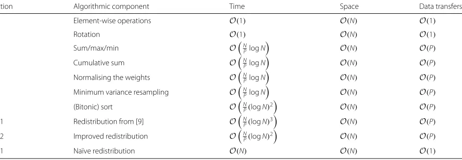
Prior to mapping the particle filter algorithm on to a MapReduce form, it is essential to understand how the operations used by a particle filter can be implemented in a fully distributed form. While a more detailed dis-cussion of these operations (and others) can be found in [26], we now discuss each of the operations that consti-tute the algorithm described in Algorithm 1. We sum-marise these operations and the associated complexities in Table 1, both for the fundamental building blocks and some of the algorithmic components that can be built from those components. Our focus is on implementa-tions with a time complexity that is as fast as possible in terms of its dependence on N, the number of data. We discuss communication complexity for each algorithmic component by considering a simplified memory architec-ture where transferring a datum between two processors is considered to be a single data movement.
4.1 Element-wise operations
Perhaps the simplest type of operation to implement in parallel involves applying an element-wise operation14. Given a functionf and a vectorv, the element-wise oper-ationf →vapplies the functionf on every element of the vector such that
f →v= f(v1),f(v2),. . .,f(vN)
In our case, normalizing the weights is an example of an element-wise operation. Another example is a vector ofif operations,Vif(a,b,c)where theith element in the output isbiifaiis true andciotherwise.
Table 1Theoretical complexities (in terms of time, space and total data transfers per unit time) of various algorithmic components of the particle filter withNdata andPprocessors
Section Algorithmic component Time Space Data transfers
4.1 Element-wise operations O(1) O(N) O(1)
4.2 Rotation O(1) O(N) O(1)
4.3 Sum/max/min ONPlogN O(N) O(P)
4.4 Cumulative sum ONPlogN O(N) O(P)
4.5 Normalising the weights ON
PlogN
4.8.2 Improved redistribution ON
P(logN)2
O(N) O(P)
It should be evident that operations that involve two inputs and a single output (e.g., element-wise sum or dif-ference) are similarly easy to implement in parallel and involves no data movement between processors.
4.2 Rotation
Another operation that we will use involves rotating (with wrapping (i.e., cyclic shift) or without) the elements of a vector by a given distance,δ, such that if the input is a
and the output isb, after the rotation, we haveb(mod(i+ δ,N))=a(i)where mod(x,y)isxmodulusy. Once again, this algorithmic component is readily parallelised with no data movements between processors.
We will also use partial rotations such that we have a vector of distances,, and not a single ‘global’ distance, δ. This vector, , has N < N elements where N is a power of two. The rotations are then implemented locally to each set ofM= NN elements. For example, if thejth ele-ment ofisδjthenb
j−1×M+modi+δj,M
= aj−1×M+ifor 1≤i≤M.
4.3 Sum, max and other commutative operations To calculate a sum of a vector of numbers, we can use an ‘adder tree’. The numbers are associated with the leaves of the tree. By recursing up the tree, the sum of the pairs of numbers can be calculated (in parallel across all pairs). The sum of all pairs of pairs of numbers can then be calculated (in parallel across all pairs of pairs). This is exemplified in Fig. 2(a–c). This process can repeat until we reach the root node of the tree and calculate the sum of all the numbers by summing the sum of the two halves of the data. See Fig. 2(d).
In fact, as has been known since the development of the infamous Array Programming Language (APL) [27], this same approach can be used for any binary operation,⊕, that is commutative such that
((a⊕b)⊕c)⊕d=(a⊕b)⊕(c⊕d) (5)
Relevant examples of operations which can be calcu-lated in this way include the sum but also the maximum (and minimum) and first non-zero element of a set of numbers (which we will denote First(.) in, for example, algorithms 2 and 3). For such operations, with N pro-cessors processing N data and a binary tree, the time complexity is the depth of the tree, i.e., log2N. Note that, near the bottom of the tree, the total communication required is proportional to the number of processors.
As should be evident, an upside-down version of the same tree can be used to implement anExpand(a) opera-tion, which involves making all elements of a vector equal to the single value ofa.
4.4 Cumulative sum
While the ability to use a tree to calculate a sum efficiently is well known, the ability to use a closely related approach to calculate a cumulative sum15efficiently appears to be less well known by researchers working on particle filters. Of course, a naïve implementation involves computing the cumulative sum by simply adding each element of the input to the previous element of the output. Such an approach would have a runtime of N. However, a more efficient approach has existed since the development of APL if not for longer16.
(a)
(b)
(c)
(d)
(e)
(f)
(g)
To ensure that the reader has some intuition as to how this could be possible, the key idea is to exploit the partial sums that are calculated in an adder tree and to express each element of the cumulative sum as a sum of these (effi-ciently calculated) partial sums. The process that exploits this insight then involves a second tree in which the values at every level are propagated to the level below, replac-ing the values that were calculated in the adder tree. More specifically, in the downward propagation, the value at each parent node is propagated to its right child and to its left child. The new value for the left child is the difference between the value at the parent node and the value at the right child node (as calculated in the adder tree). The new value for the right child is just the same value as the parent node. See Fig. 2(e–g) for an example.
With this forward and backward pass of the tree, we can obtain the cumulative sum in 2 log2Nsteps.
4.5 Normalising the weights
Normalising the weights is an example of an opera-tion that can be implemented using the building blocks described to this point. The sum is calculated using an adder tree (as described in Section 4.3), distributed to all the data (as also described in Section 4.3) and an element-wise divide (see Section 4.1) used to calculate the normalised weights.
4.6 Minimum variance resampling
As explained in Section 3.3, resampling involves deter-mining the number of copies of each particle that are needed. We specifically describe minimum variance resampling, for which the number of copies of the ith particle is
mi= Ci×N − Ci−1×N +1 (6)
wherexandxare respectively the ceiling17 and the floor18ofx, where
Ci= (6) uses only element-wise operations (as described in Section 4.1) and a rotation (by a single element and as described in Section 4.2). (7) involves a cumulative sum (as described in Section 4.4) and an addition (as described in Section 4.1). Thus, the building blocks described to this point can be used to implement (6) and (7).
4.7 Sorting
Quicksort [28] is well known and has an average time complexity of O(Nlog2N). However, we focus on the bitonic sort algorithm [29], which has a time complex-ity ofONP log2N2and a spatial complexity ofO(N).
The number of data movements at each iteration isP. The main reason for this choice is that we want to guarantee the time taken to perform sorting. While it is possible to parallelise quicksort, the ability to do so is data dependent. In contrast, bitonic sort has deterministic time complexity (with a balanced load across (up to)Nprocessors).
At the fundamental level, abitonic sequenceforms the basis for the bitonic sort. A sequencea= [a1,a2,. . .,aN] is a bitonic sequence ifa1 ≤a2 ≤ . . . ≤ak ≥ . . .≥ aN for somek, 1 ≤ k ≤ N or if this condition holds for any rotation ofa.
To try to provide some intuition as to how the algorithm works, note that at a certain point it the algorithm, we have N data in a bitonic sequence. The first ‘half ’ of the data are sorted in an ascending order and the second half are sorted in a descending order19. Consider theith element in the first half and the ith element in the second half. There are N2 −1 data between these two elements. They must all be larger than the smallest of the two elements which the data are between. There must therefore be at least N2 data that are larger than the smallest of the two elements. This smallest element must therefore be one of the lowest N2 data (it cannot be one of the largest N2 data if there are at leastN2 data larger than it). An upside-down version of the same argument makes clear that the largest of these two elements must be one of the largest N2 data. Finally, it also transpires that after this operation, the first
N
2 data are a bitonic sequence and the secondN2 data are a bitonic sequence. Thus, given a bitonic sequence, by com-paring all pairs of data that are a distance of N2 apart and swapping the points if needed, we can ensure all the larger elements are in the first N2 data, which forms a bitonic sequence, and all the smaller elements are in the second
N
2 data, which also forms a bitonic sequence. We can then apply the same comparison structure on each of the two bitonic (smaller) sequences. This process can be applied recursively until pairs of points are compared and the data are sorted.
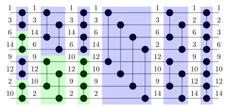
An example of bitonic sort with eight numbers is pro-vided in Fig. 3.
4.8 Redistribution
4.8.1 Original version from [9]
The redistribution algorithm takes two inputs, the old population of particles x and the number of copies m, and produces the new population of particles,x∗, as the output.
In [9], a divide-and-conquer algorithm was described for implementing the redistribute. The procedure involves sorting the particles in decreasing order of the number of copies. With N data, the sum of the elements of m
must beN. The approach is then to divide the data into two smaller datasets, each of which has N2 elements and is such that the corresponding elements ofmare sorted and sum to N2. This can be achieved by finding thepivot, which we define as the leftmost element inmfor which the associated value of the cumulative sum isN2 or greater. In general, the pivot needs to be split into two constituent parts such that the two smaller datasets can both sum to
N
2. We refer to these two parts as the left pivot and right pivot. The data to the left of the pivot and including the left pivot can be used to produce one of the two smaller datasets. The right pivot and the data to the right of the pivot can be used to produce the other of the two smaller datasets. Both smaller datasets are then sorted21such that they are in decreasing order ofm. Note that there is a spe-cial case that occurs when the value of the right pivot is zero: the rotation needed is one less than otherwise in this case. It can be intuitive to think of this procedure as oper-ating on a tree. Applying the procedure recursively down the tree, until the leaf nodes are encountered, results in the redistribute completing. See Fig. 4 for an illustrative example of this procedure.
A few points are worth highlighting: the operation of the algorithm is not dependent onmand not dependent on the distribution of the weights; sort can (somewhat counter intuitively and seemingly unnecessarily) change
Fig. 3Example of bitonic sort using eight numbers. Each horizontal wire corresponds to a core. The blue color denotes that the larger value will be stored at the lower wire after the comparison, while the green color the opposite
the order of numbers in a list when elements of the list are not unique; if no copies of a particle are to be generated, the identity of the corresponding particle is irrelevant to the eventual output of the algorithm.
The procedure can be described using element-wise operations (see Section 4.1), sum (see Section 4.3), cumu-lative sum (see Section 4.4), rotations (see Section 4.2) and sort (see Section 4.7). Algorithm 2 provides a description of this algorithm. Note that the description makes use of three functions (LeftHalf(.),RightHalf(.)andCombine(.)) which are included to aid exposition (and actually have zero computational cost). Also note that the implemen-tation is described in a way that involves recursion. It is possible to ‘unwrap’ the recursive implementation such that all operations (at all stages in the tree) are imple-mented on datasets of the same size (a size ofN). Doing so is conceptually straightforward though the bookkeeping required is non-trivial.
Algorithm 2 Redistribute: O(NP(log2N)3) implementa-tion.
1: Function x=Redistribute(m,x)
2: m: Number of copies (sorted in descending order) 3: x: Particles
4: ifLength(m) >1then
5: Calculate Cumulative Sum
6: c←CumSum(m)
7: Identify Pivot
8: ip←First(c≥ N2)
9: p←Expand(ip)
10: Calculate Left-Pivot and Right-Pivot
11: i simply indexes the elements of m and0 is a vector of zeros
12: lp←Vif(i=p,c− N2,0)
13: rp←Vif(i=p,N2 −Rotate(c, 1),0)
14: Generate Smaller Datasets
15: l←LeftHalf(Vif(i<p,m,lp))
16: lx←LeftHalf(x)
17: r←Vif(i>p,m,rp) 18: Calculate Rotation ofr 19: inc←Sum(Vif(c= N2,1,0))
20: r←RightHalf(Rotate(r,ip+inc))
21: rx←RightHalf(Rotate(x,ip+inc))
(a)
(b)
Fig. 4An example of the redistribution forx=[10, 9, 12, 6, 1, 3, 14, 2] andm=[4, 2, 1, 1, 0, 0, 0, 0] using the original and improved (new) redistribute. The original redistribution always sorts the number of copies vector (bottom vector) in a descending order, while this is not required in the new redistribution (e.g., see node no. 3).aOriginal.bNew
The time complexity of this redistribution algorithm
ON
P(log2N)3
in parallel with N processors since a (bitonic) sort (with complexity ofONP(log2N)2) is used at each stage in the divide-and-conquer. Note that this contradicts the (erroneous) claim in [9] that the time complexity of this algorithm isONP(log2N)2. The com-munication complexity is (again)P.
4.8.2 Improved redistribution
The redistribution algorithm described in Section 4.8.1 is a divide-and-conquer algorithm that ensures that, at each node in the tree,msums to its length,N, and is sorted. The sorting is sufficient to ensure that rotation can be used to replace some of the (rightmost) zeros with the (rightmost) non-zero elements ofmthat sum toN2.
Here we exploit the observation that it is possible to define an alternative divide-and-conquer strategy. More specifically, we ensure that, at each node in the tree,m
sums to its length,N, and has all its non-zero values to the left of all values that are zero. Since such a sequence only has trailing zeros, we call such a sequence an All-Trailing-Zeros (ATZ) sequence22. While a sort is sufficient to generate an ATZ sequence, it is easier, as we will demon-strate shortly, to generate an ATZ sequence than it is to generate a sorted sequence.
The new algorithm, at each node in the tree, starts with
m, which sums to its length,N, and is an ATZ sequence. To proceed, as previously, we find the pivot (as defined in Section 4.8.1). As previously, the data to the left of the pivot and the left pivot can be used to produce one of the two smaller datasets. However, in contrast to the approach described in Section 4.8.1, we can simply use the right pivot and the data to the right of the pivot to generate the second smaller dataset (without any need for sort). Both these smaller datasets then sum to N2 and are ATZ sequences. Note that, as with the approach described in Section 4.8.1, there is a special case that occurs when the value of the right pivot is zero.
To initiate the algorithm, we need to generate an ATZ sequence. To achieve this, we propose to use (bitonic) sort (once). After this initial sort, the procedure can be described using element-wise operations (see Section 4.1), sum (see Section 4.3), cumulative sum (see Section 4.4) and rotations (see Section 4.2). We emphasise that there is no need for a sort after the initial generation of an ATZ sequence. As a result, while the algorithm described in Section 4.8.1 has time complexity ofONP(log2N)3, the algorithm described in this section has time complex-ity of ONP(log2N)2. Notice that the number of data movements is stillP. To aid understanding, algorithm 3 provides a description of this algorithm. Note the very strong similarity to algorithm 2 and that, once again, it is possible to ‘unwrap’ the recursive implementation albeit with some non-trivial bookkeeping.
5 Mapping particle filtering into MapReduce The descriptions provided in the Section 4 describe dis-tributed operations that can manipulate vectors (albeit after some unwrapping of the recursive descriptions).
As discussed in the Section 2.2, the fundamental notion of MapReduce is the processing of (key, value) pairs. In the context of particle filtering, none of the properties of the particles (weight or state) qualifies to be a key. However, we can give each particle a unique index and use this index as the key, such that we think of the particles as being a set{i,xi,wi}wherei∈ {1,. . .,N}and, as previously men-tioned, whereNis the number of particles,xiis the state andwiis the corresponding weight of theith particle.
6 Evaluation
Algorithm 3 Redistribute: ONP(log2N)2
implementa-5: Calculate Cumulative Sum
6: c←CumSum(m)
7: Identify Pivot
8: ip←First(c≥ N2))
9: p←Expand(ip)
10: Calculate Left-Pivot and Right-Pivot
11: i simply indexes the elements of m and0 is a vector of zeros
12: lp←Vif(i=p,c− N2,0)
13: rp←Vif(i=p,N2 −Rotate(c, 1),0)
14: Generate Smaller Datasets
15: l←LeftHalf(Vif(i<p,m,lp))
16: lx←LeftHalf(x)
17: r←Vif(i>p,m,rp) 18: Calculate Rotation ofr 19: inc←Sum(Vif(c= N2,1,0))
standard estimation problem (involving a scalar state and a computationally inexpensive proposal, likelihood and dynamic model) that is widely used in the particle filter-ing community [20]. We perceive this scenario emphasises the need for efficient resampling, where, as is often the case, the likelihood, dynamics and proposal were compu-tationally demanding and the relative merits of different
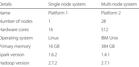
Table 2Details of the experimental platform used for evaluation
Details Single node system Multi-node system
Name Platform 1 Platform 2
Number of nodes 1 28
Hardware cores 16 512
Operating system Linux IBM Unix
Primary memory 16 GB 384 GB
Spark version 1.6.2 1.4.1
Hadoop version 2.7.2 2.7.1
resampling schemes would be less apparent. Our evalu-ation focused on specific aspects of the implementevalu-ation, which are described as follows:
1. We start, in Section 6.1, by providing evidence that, in contrast to a naïve implementation, the particle filter we have developed can exploit multi-core architectures while having deterministic runtime. 2. In Section 6.2, as a precursor to a detailed evaluation
and analysis, we analyse the overall profile of the particle filtering algorithm for implementations on a single core, using Hadoop and using Spark.
3. Then, in Section 6.3, for both the Spark and Hadoop implementations, we compare the performance of our new algorithms relative to a single mapper and a single reducer. In doing so, we not only compare the overall performance, but we also compare the fundamental building blocks of the particle filtering algorithm. This section provides a thorough understanding of these algorithms’ performance on two key frameworks that support MapReduce. 4. Given that the Spark implementation
(unsurprisingly) outperforms the Hadoop implementation, we then focus on the Spark
implementation. In Section 6.4, we then compare the two versions of the redistribution algorithm
described in Sections 4.8.1 and 4.8.2 as a function of the numbers of particles and cores. The intent is that this detailed comparison provides insight into the performance that is achievable using the original and proposed variants of the redistribution algorithm. 5. Finally, in Section 6.5, we perform a detailed analysis
on the speedup and scalability of the redistribution and the overall particle filter.
In performing these evaluations, a basic parameter that we found useful in assessing the algorithmic performance is the capability to process large amount of data, which directly translates to the number particles that can be pro-cessed per unit time, the number of particles propro-cessed per second (PPS).
6.1 Worst-case runtime performance 6.1.1 Baseline redistribution algorithm
population, we can populate the new generation of parti-cles (Algorithm 4). In MapReduce, a map function is used for the outer for loop and within each map, we iterate as many times as needed according to the number of copies elements.
Algorithm 4Redistribute:O(N)implementation. 1: Functionx∗=Redistribute(m,x)
2: m: Number of copies 3: x: Particles
4: x∗: New population of Particles 5: i←0
6: forj=0toNdo 7: fork=0tom jdo
8: New Population of Particles 9: x∗[i]←x[j]
10: i←i+1 11: end for 12: end for 13: EndFunction
Note that this algorithm, when running across multiple cores, can be expected to have a runtime complexity that is dependent on the data. To help make this clear, consider the worst case where the redistribution involves makingN copies of theith particle (and zero copies of all other parti-cles). In this case, only one core will actually be populating the new generation of particles.
6.1.2 Runtime performance and variability
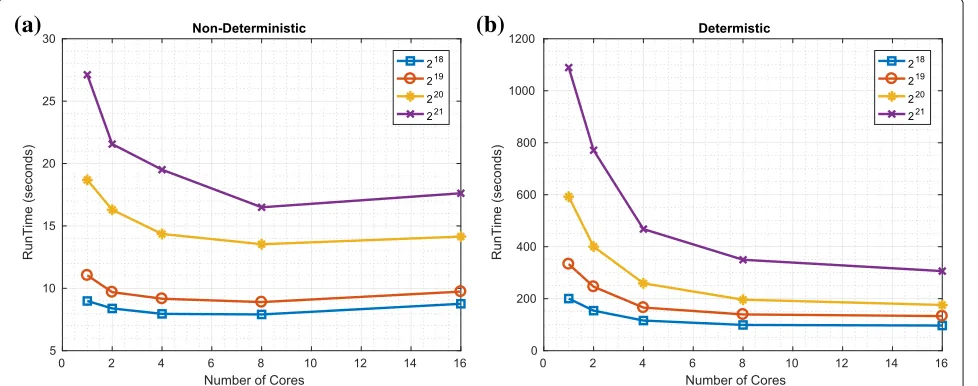
We investigated the worst-case performance of such a naïve parallel implementation of the redistribution com-ponent and compared with our proposed implementation
(using a Spark implementation). The results are shown in Figs. 5 and 6 for the worst case (where the new popula-tion of particles are all copies of a single member of the old population). It should be evident that as the number of cores increases, the runtime of the proposed (almost) never increases23. In contrast, while the runtime of the naïve implementation initially decreases as the number of cores is increased, it then increases (i.e., such that it is faster in absolute terms to use 8 not 16 cores with platform 1 and such that it is faster to use less than 50 cores not 512 cores with platform 2). The reason for the decrease is that the MapReduce framework can use the extra cores to more rapidly process the (many) zeros in the vector describing the number of copies. The reason for the subsequent increase in processing time is that the additional overhead of having multiple cores becomes increasingly significant if only one of the cores is doing the vast majority of the processing.
It should also be evident that the absolute runtime (on these platforms and with our current Spark implementa-tion) of the deterministic and non-deterministic variants differ significantly such that the naïve implementation can be approximately 20 times faster (in the contexts of both platforms). This is disappointing and does motivate future work to refine our (initial) implementation. However, we perceive that there are applications where a slower but deterministic runtime is preferable to a faster but data-dependent runtime. In the contexts of such applications, particularly given the scope to improve the implemen-tation, we perceive our algorithm (if not our current implementation) has utility.
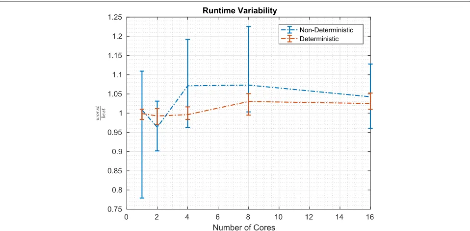
To assess the variation in runtime that we experience empirically when considering different distributions of the weights, we compared the performance in the context of
(a)
(b)
(a)
(b)
Fig. 6Worst-case performance of redistribution: platform 2.aNaïve implementation.bProposed approach
the worst-case scenario with the performance in the best-case scenario24. Figure 7 describes the average runtime (as well as the minimum and maximum runtimes) over five runs. It is immediately clear that the fluctuations between the runs are smaller in the context of the deterministic than in the context of the naive non-deterministic algo-rithm. What is perhaps less clear, but still discernable, is that the average runtime for the deterministic redis-tribute is impacted less by moving from the worst-case to the best-case scenario than the naive non-deterministic redistribute. We believe that this modest difference
points to the runtime being dominated by things other than the algorithmic choice: for example, MapReduce’s overheads (which are common to both algorithms’ implementations).
6.2 Overall profile
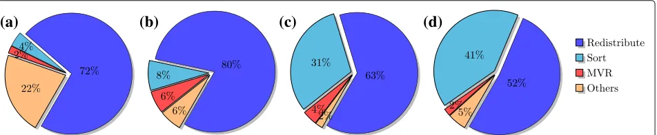
We now compare performance of three implementations of a particle filter: a sequential implementation (in Java and using quicksort in place of bitonic sort), an imple-mentation in Hadoop and an impleimple-mentation in Spark. All implementations involve a single core and platform 1.
Figure 8 shows the proportion of the runtime that is associated with redistribution, sort, minimum variance resampling (MVR) and the remaining components (e.g., sum, cumulative sum, diff, scaling).
As can be observed from Fig. 8, the majority of the time taken is devoted to the redistribution component. Note that, for the Spark implementation, a significant fraction of the remaining time is spent on the sorting component and the fraction of time devoted to redistri-bution and sorting increases as the number of particles is increased.
6.3 Comparison of Hadoop and Spark
We next investigate how the choice of middleware impacts performance in the context of the components of the algorithm and in the context of the entire particle filter algorithm. All implementations involve a single core and platform 1.
6.3.1 Sum and cumulative sum
Figure 9 shows the comparative performance of the sum and cumulative sum components in these two key frame-works.
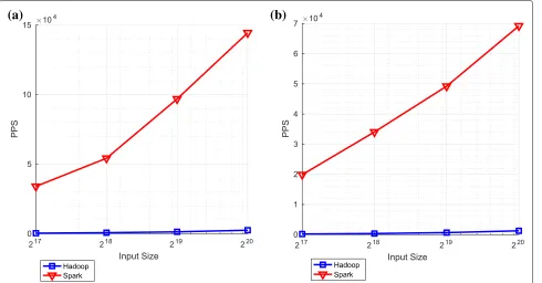
With respect to the number of particles processed per second (PPS), the performance using Spark is far superior to that achieved using Hadoop. This stems from the issues discussed in Section 2: Spark uses RDDs to makes use of memory (and lazy evaluation) whereas Hadoop only uses the file system (HDFS) to transfer data from the output of one operation to the input of the next.
It is apparent in both frameworks (and particularly apparent in the context of Spark) that, as the number of particles increases, the number of particle processed per second also increases. This is because with more particles, the overheads associated with setting up (and tearing down) the mappers and reducers are increasingly offset by the parallel operations that make use of the mappers and reducers. The limited extent to which this effect is observed in the context of Hadoop highlights that the overheads associated with opening files in HDFS are significant.
Since, as explained in Section 4, calculating a summa-tion involves one adder tree and cumulative sum involves two such trees, we should expect the number of particles per second for the cumulative sum to be approximately half that for the summation. A comparison of the two graphs in Fig. 9 makes clear that this is indeed (approx-imately) the case for both frameworks and for all input sizes.
6.3.2 Bitonic sort and minimum variance resampling Figure 10 shows the performance for two independent components,bitonic sort andminimum variance resam-pling. The performance ofminimum variance resampling is relatively close to the performance of the cumulative sum (see Fig. 9). This is expected since, as explained in Section 4, minimum variance resampling includes a cumulative sum.
Once again and for the same reasons as discussed in Section 6.3.1, we notice the same difference in perfor-mance between the Spark and Hadoop implementations. As one might expect and as before, forminimum variance resampling, the number of particles per second increases with the number of particles. However, it is noteworthy that, for bitonic sort with Spark, the number of parti-cles per second decreases for large numbers of partiparti-cles. On investigating this in some detail, we observed that the lineagesused to facilitate the lazy evaluation in Spark25 become very large with large numbers of particles. This appears to cause Spark to become less efficient when the number of particles becomes large.
6.3.3 Redistribution and overall performance
Finally, Fig. 11 shows the comparative performance of the redistribution algorithm (as described in Algorithm 3) and the overall particle filtering algorithm.
Once again, we notice the same differences between Hadoop and Spark. In the context of the overall parti-cle filter and for the largest number of partiparti-cles consid-ered, these differences are manifest in Spark, relative to Hadoop, offering a considerable speedup (approximately 25-fold26).
(a)
(b)
(c)
(d)
(a)
(b)
Fig. 9Summation and cumulative summation on Spark and Hadoop.aSummation.bCummulative summation
The overall performance of the particle filtering algo-rithm, when implemented in Spark, decreases for large numbers of particles. Again, on investigation, this appears to be caused by large lineages associated with the large number of particles. Finally, we note that the bitonic sort and redistribution components appear to be limiting the
number of particles per second that can be processed by the overall particle filtering algorithm.
6.4 Impact of using multiple cores
We now focus on the Spark implementation (with plat-form 1) and compare the perplat-formance of the two variants
(a)
(b)
(a)
(b)
Fig. 11Redistribution and the overall particle filtering on Spark and Hadoop.aRedistribution.bOverall particle filtering
of the redistribution component in isolation and in the context of the overall performance of a particle filter. More specifically, we investigate how performance scales with the number of cores and the number of particles.
6.4.1 Redistribution component in isolation
Figure 12 compares the performance of the two versions of the redistribution component as a function of the number of particles and number of cores.
On a core-to-core basis, theOlog2N2
redistribu-tion component outperforms theOlog2N3
compo-nent across all numbers of particles by a margin of up to a factor of approximately 4 (for 16 cores).
For all numbers of particles, increasing the number of cores improves performance for both variants of the redis-tribution component. However, in the context of both variants, the improvement in performance when consid-ered as a ratio is less than the ratio of the number of cores.
In the context of theO
ing the number of particles for a fixed number of cores can significantly reduce the number of particles processed per second. This is not the case for theONP log2N2 of particles while keeping the number of cores constant improves the number of particle processed per second. However, in the context of theO
increasing the number of particles for a fixed number of
cores can reduce the number of particles processed per second.
6.4.2 Resulting overall particle filter performance
Figure 13 compares the performance of the original parti-cle filtering algorithm when using the two variants of the redistribution component.
The comparative performance that was observed in the context of the redistribution component in isolation is also evident when comparing the performance of the overall particle filter. Indeed, the use of theONP(log2N)2
variant of redistribution results in (approximately) a fourfold increase in the number of particles processed per second. The trends that were observed in the context of the redistribution component in isolation are also apparent in the context of the overall particle filter.
6.5 Speedup and scalability analysis
We now focus on the speedup that the ONP(log2N)2
variant of the redistribution component offers relative to the ONP(log2N)3
variant and the scalability of the
ON
P(log2N)2
variant, i.e., the extent to which using more cores improves performance.
(a)
(b)
Fig. 12Performance of the two variants of the redistribution component (using Spark).aRedistributionON P(log2N)2
.bRedistribution
ON P(log2N)3
(a)
(b)
We compare performance in the context of both plat-forms for various different numbers of particles.
6.5.1 Redistribution component in isolation
Figures 14 and 15 describe the speedup and scalability of the ONP(log2N)2
redistribution component in the context of platforms 1 and 2 respectively.
We note that the relative speedup of theONP(log2N)2
variant of the redistribution component (relative to the
ON
P(log2N)3
variant) is significant in all cases: between 2 (on platform 1) and 24 (on platform 2). For both plat-forms, this speedup increases as the number of particles is increased. However, we also note that, with platform 1 (which has a single node such that all cores share mem-ory), the speedup decreases as the number of cores is increased for a fixed number of particles. In contrast, with platform 2, the speedup is broadly constant for large numbers of cores.
We also note that the scalability of theONP(log2N)2
variant of the redistribution component is far from ideal: increasing the number of cores culminates in minimal (if any) improvements in performance. This occurs because, in the context of both platforms, it is the com-munication, and not the computation, that is limiting performance. This also explains why platform 2’s larger number of cores does not offer improved scalability
relative to platform 1: in platform 2, the processors are distributed across multiple nodes and communicate across a network, whereas platform 1’s processors are all part of the same node and so communicate using shared memory.
6.5.2 Resulting overall particle filter performance
Figures 16 and 17 describe the speedup and scalability of the overall particle filter using theONP(log2N)2
redis-tribution component in the context of platforms 1 and 2 respectively.
The speedups, as measured in the context of the overall particle filter algorithm are between 3 and 9.5. Again, for both platforms, the speedup increases with the number of particles. Again, the scalability is far from ideal.
6.6 Discussion
The goal of the research is to dramatically reduce the exe-cution time of particle filters. While we have gained sig-nificant insights from the performance analysis described herein (and hope that the paper will help others to also capitalise on those insights), the results described herein are ultimately disappointing: using the combination of algorithms and hardware considered herein, we are unable to improve on the execution speed achieved by a naïve redistribute implementation.
(a)
(b)
Fig. 14Relative speedup and scalability of theONP(log2N)2variant of the redistribution component on platform 1.aRelative speedup:
ON
(a)
(b)
Fig. 15Relative speedup and scalability of theONP(log2N)2
variant of the redistribution component on platform 2.aRelative speedup:
ON P(log2N)2
.bScalability:ONP(log2N)2
(a)
(b)
Fig. 16Relative speedup and scalability of the overall particle filter algorithm using theONP(log2N)2variant of the redistribution component on platform 1.aRelative speedup:ONP(log2N)2
(a)
(b)
Fig. 17Relative speedup and scalability of the overall particle filter algorithm using theONP(log2N)2variant of the redistribution component on platform 2.aRelative Speedup:ONP(log2N)2.bScalability:ONP(log2N)2
At one level, this is because the baseline against which we are comparing performance is relatively simple and mature. Our corresponding implementation is therefore relatively well optimised. In contrast, our proposed imple-mentation is novel and has not been significantly opti-mised. However, we do not see it as fruitful to optimise our current implementation: we believe the disappointing results are caused by two other issues.
The first issue is that, in our implementations, we have assumed that each particle has a unique key in the MapRe-duce framework. There are therefore as many keys as there are particles. To understand the potential benefit of having more than one value per key, we investigated how the performance of summation (in the context of a single core in platform 1 and 220values) changes as a function of the number of values per key. Figure 18 highlights that, for the example of summation in the context of a specific hardware configuration, a fourfold improvement in exe-cution speed is possible by changing the number of values per key. This implies that runtime could change signifi-cantly if other components considered multiple particles to be associated with each key.
However, the primary issue which appears to be limit-ing runtime is the very MapReduce framework itself. As discussed in Section 2.2, before every Reduce operation, the values associated with each key are collated. This
is a useful feature in the context of applications where the number of values associated with each key and the number of unique keys are unknown (e.g., where the task is to count up the number of occurrences of each word in a set of documents). However, in the particle filter
considered herein, the number of unique keys is known to be the number of particles and the algorithms are chosen such that the number of values for each key are pre-defined for each algorithmic component. The flex-ibility that MapReduce provides is therefore of no utility in the context of the particle filter implementation. That lack of utility is not per se an issue. What is an issue is that the flexibility is achieved through a (somewhat hid-den) ‘shuffle-and-sort’ phase that precedes every reduce operation. This phase (self-evidently from the name) in the versions or frameworks we used, was single-core bound. This sort is demanding in terms of communi-cation and processing. So, every time MapReduce is used to perform even simple operations (e.g., cumulative sum), it is likely that the infrastructure is actually col-lating the keys and sorting them. Given the number of simple operations involved in our particle filter opera-tion, we perceive it is this overhead that is dominating execution time.
This paper therefore motivates consideration of alter-native frameworks which do not provision for the same flexibility as MapReduce and therefore do not have the same overheads. Our future work will therefore consider rethinking the entire manifestation of the implementation in alternative lower-level frameworks (e.g., using Message Passing Interface (MPI), a framework designed for HPC applications).
7 Related work
A review of different resampling techniques is provided in [33]. This review makes clear that, at first sight, some of the key components of a particle filter, notably cumulative sum and redistribution, are inherently sequential28.
Indeed, this thinking has motivated research (e.g., as described in [44]) into approaches where a (small) number of processing elements (PEs) each perform local resam-pling and then communicate via a central process that, for example, allocates the particles to the PEs (a process that, as demonstrated in section 6, results in non-deterministic runtime). In contrast to the approaches involving com-munication between PEs, this paper is focused on a fully distributed algorithm (with no explicit central pro-cess and so no implicit assumption of a small number of PEs).
The detailed comparison of different (single-processor implementations of ) resampling algorithms provided in [43] highlights that systematic resampling offers the best performance amongst the approaches considered. One strategy for parallel implementation (discussed in [44] and explored in more detail elsewhere [32]) is to deliberately choose an alternative resampling algorithm such that the alternative algorithm is more amenable to parallel imple-mentation. This paper focuses on systematic resampling specifically.
Another approach that [33] highlights involves each par-ticle performing resampling using only information from its local neighbours (e.g., as described in [34], which, in the view of the authors, does not make obvious that, if the resampling is performed locally then the weight after resampling should be proportional to the local nor-malising constant29). In contrast to approaches based on considering only local neighbours, this paper describes approaches that provide exactly the same output as a single processor would have generated.
Research not explicitly covered in the aformentioned review includes the implementation described in [9] and which this paper explicitly builds upon. That implemen-tation achieves ONP(logN)3 time complexity with N parallel processors (and achieves a runtime that is not data dependent). Other related research includes (in [35]) a more complex, parallelised particle filter that uses a context-aware scheduling algorithm. They address the load imbalance arising from the naïve parallelisation of the particle filtering by using a custom (but reusable) scheduler. In this paper, we replace the use of such a scheduler at runtime by algorithmic development at design-time.
There has been previous work on implementing particle filters in a MapReduce context (e.g., in [7, 8]). How-ever, this research has focused on using Hadoop and has not included a similar analysis to that documented in Section 6 of this paper. Our analysis in that section of this paper indicates that substantial improvements are possible using Spark but also highlights that the speedup offered using MapReduce and large numbers of proces-sors is somewhat disappointing.
8 Conclusions
In this paper, we have developed an improved paral-lel particle filtering algorithm. The core novelty is a novel redistribution component. The component pro-vides deterministic runtime and a time complexity of
ON
P(logN)2
(withN particles andNprocessors). This improves on a previous approach that achieved a time complexity ofONP(logN)3.
that, as the number of particles increases, so does the implementation efficiency.
This performance evaluation highlights that it is not always valid to assume that porting algorithms to Big Data frameworks will result in an increase in execution speed. Indeed, the implementation we evaluated is limited by the communications overhead necessarily associated with giving each particle a unique key in the MapReduce framework: as a result, while we can achieve a speedup of threefold with 16 cores in a single node, with 512 cores spread across 28 nodes, we only achieve a speedup of approximately 1.4 (i.e., less). Furthermore, our implemen-tation is outperformed by a naïve implemenimplemen-tation by a factor of approximately 20. Put simply, using our current implementation, we cannot yet outperform an (optimised) single-processor resampling algorithm.
Of course, there will be applications where resampling is a small fraction of the total computational cost of the particle filter. In such contexts, the proposal, likelihood and/or dynamic model will be computationally demand-ing to calculate. These components of the particle filter are trivial to parallelise. Our future work will aim to broaden the applicability of our results beyond those applica-tions. More specifically, we plan to focus on architectures involving a single key being related to multiple particles, explicitly minimising the need for data movement and removing the large lineages that appear to be limiting the performance possible using Spark.
Finally, we note that we have made our implementations available for public access via an OpenSource repository at GitHub asparticlefilter[30].
Endnotes
1Though we are not aware of any empirical analysis of
this approach being published.
2More specifically, the algorithm’s runtime is
indepen-dent of the distribution of the weights in the particle filter.
3Including the associated ever-growing ecosystem of
tools (e.g., Mahout [31] and GraphX for Spark [36]).
4Conventional High Performance Computing (HPC)
approaches use parallel computations to optimise pro-cessing time. We refer the reader to [37] for a good coverage of HPC-bound approaches for parallelising applications.
5We anticipate that the ‘heat wall’ (i.e., the inability to
remove enough heat from transistors that switch ever faster) will mean that for chip manufacturers to meet the expectation set by Moore’s law, they will soon (if not already) be doubling the number of cores (not transistors per square inch) used in each processor each year. In ten years’ time, if this trend continues, we would have desktop
computers with a thousand times as many cores as today. This trend motivates the authors to design implementa-tion strategies for particle filters that are well suited to the multi-core processors which will, we believe, become increasingly prevalent over time.
6This contrasts HPC-based solutions, where the
pro-grammer aims to exploit intricate knowledge of the underlying architecture to ensure that data movement and processing are jointly optimised for the specific hard-ware.
7The exact number of mapper and reducer processes
on a parallel resource (for instance, a multi-node cluster) varies depending on the configuration, but the impor-tant point is that the algorithm developer does not need to worry about how the processes are distributed when defining the algorithm. Of course, that does not mean that there is not utility in the developer describing algo-rithms using mappers and reducers that are well suited to the problem being tackled and to the configuration being used.
8Note that the output from each sentence would only be
for the words that occur in that sentence, not every word that ever occurs in the corpus.
9This can make it hard for a programmer to debug
algo-rithmic implementations, particularly if the programmer is unfamiliar with debugging software performing lazy evaluation.
10While the derivation involves consideration of a path,
the resulting algorithm only needs to store the most recent state.
11A good choice of proposal density can delay but not
stop the effect [22].
12This, of course, leads to a loss of diversity among the
particles.
13For instance, although Quicksort [28] can be
par-allelised, the load distributions across the processors is dependent on the pivots used and the run-time will there-fore be data-dependent.
14Such operations are an example of ‘embarrassingly
parallel’ operations that are arguably trivial to parallelise.
15Note that the cumulative sum is sometimes referred
to as a prefix sum: there is no difference between a prefix sum and a cumulative sum.
16APL describes an approach to calculating a sum,

![Fig. 4 An example of the redistribution for x = [10, 9, 12, 6, 1, 3, 14, 2] and m = [4, 2, 1, 1, 0, 0, 0, 0] using the original and improved (new) redistribute.The original redistribution always sorts the number of copies vector (bottom vector) in a descen](https://thumb-us.123doks.com/thumbv2/123dok_us/882591.1106047/9.595.58.542.86.225/example-redistribution-original-improved-redistribute-original-redistribution-vector.webp)