Mapping Quantitative Trait Loci Using Generalized Estimating Equations

(1)



Mapping Quantitative Trait Loci Using Generalized Estimating Equations

Christoph Lange*

,†

**_{and John C. Whittaker*}**

*School of Applied Statistics, University of Reading, Reading RG6 6FN, United Kingdom and†_{Department of Biostatistics,}

Harvard School of Public Health, Boston, Massachusetts 02115 Manuscript received November 17, 2000 Accepted for publication August 29, 2001

ABSTRACT

A number of statistical methods are now available to map quantitative trait loci (QTL) relative to markers. However, no existing methodology can simultaneously map QTL for multiple nonnormal traits. In this article we rectify this deficiency by developing a QTL-mapping approach based on generalized estimating equations (GEE). Simulation experiments are used to illustrate the application of the GEE-based approach.

O

VER the last 10 years, there has been a great deal data (LiangandZeger1986;Diggleet al.1996). The advantage of the GEE methodology is its semiparametric of interest in the development of methodology to

map quantitative trait loci (QTL) relative to a known character: Correct specification of the mean and covari-ance structure of the model is sufficient to guarantee marker map in populations derived from inbred line

crosses. Perhaps the most commonly used current tech- asymptotically unbiased parameter estimates, regardless of the actual underlying probability model. In fact, esti-niques for univariate traits are based on the work of

Jansen(1994) andZeng(1994). These assume a normal mation of mean parameters (we see below that these include the QTL location and effect) is also robust to distribution for the environmental errors and solve the

resulting likelihood equations via the expectation-max- misspecification of the covariance structure, although efficiency of estimation is higher the better specified imization (EM) algorithm (Dempsteret al.1997). These

methods naturally extend to simultaneous QTL map- the covariance structure is.

In this article we concentrate on F2 populations, but

ping of several normally distributed traits (Jiangand

Zeng1995). This is useful because when the environ- the proposed methodology can easily be applied to any genetic design; we need only derive appropriate mean mental correlation structure is modeled properly,

simul-taneous QTL mapping improves the efficiency of pa- and variance assumptions for the design of interest. rameter estimates (Korol et al. 1995; Henshall and

Goddard1999). Furthermore, pleiotropic effects can

METHODS be included and estimated. Analogues of these methods

based on least-squares also exist (Haley and Knott _{We begin by introducing the GEE concept. We can} 1992;Martı´nezandCurnow1992;KnottandHaley _{give only an intuitive motivation of the concept here;} 2000) and in most, although not all (Xu 1995; Kao _{more formal treatments can be found in}_McCullagh 2000), situations give very similar results to the likeli- _and _Nelder _(1989), _Diggle _{et al.} _{(1996), or} _Heyde hood-based methods, with reduced computational com- _(1997).

plexity (KnottandHaley2000). _{Consider a vector of responses}_Y_{such that the} expecta-In contrast, relatively little work has been done on _{tion of}_Y_{can be written}_E(_Y₎_{⫽ ␮}₍_␥_{) for some function} mapping procedures for nonnormally distributed traits _␮_{, where}_␥_{is a vector of parameters we wish to estimate.} (but see Hackett and Weller 1995; Visscher et al. _{Intuitively, a sensible way to do this would be to choose}_␥_ˆ 1996a,b;HenshallandGoddard1999). In particular, _{to make}_Y_{⫺ ␮}₍_␥_{) “small.” We might therefore consider} no methods map QTL of several correlated nonnormally _{choosing estimates of} _␥_{ˆ that solve the set of equations} distributed traits simultaneously. This may be because

A(Y⫺ ␮(␥ˆ))⫽ 0 (1)

of the difficulty in specifying a full probability model for such data: This makes likelihood-based approaches

for a suitably chosen matrixA. In fact, it can be shown difficult to implement.

that in many situations the optimal choice of A isDT

Here we avoid these difficulties by using the

general-V(␮, ␣)⫺, where V(␮, ␣) is the covariance matrix for ized estimating equation (GEE) approach to correlated

Y, which may depend both on the mean and on a vector of other parameters␣, and the matrix of derivativesDis given byDir⫽⳵␮i/⳵␥r. This can be shown to give consistent

Corresponding author:Christoph Lange, Department of Biostatistics,

estimates of ␥ that are highly efficient relative to

full-Harvard School of Public Health, 655 Huntington Ave., Boston, MA

02115. E-mail: [email protected] likelihood methods for many underlying probability

(2)

1326 C. Lange and J. C. Whittaker

TABLE 1

Typical link and variance functions

Trait type Link functionh(␮)⫽ Distribution Range φ Variance functionV(␮)

Continuous ␮ Normal ⺢ ␴2 ₁

Count ln(␮) Poisson ⺞0 1 ␮

Proportion ln

冢

␮

1⫺ ␮

冣

Binomial {1, . . . ,n} 1

n ␮(1⫺ ␮)

Positive continuous _␮1 Gamma ⺢⬎0

1

␯ ␮2

Inverse Positive continuous 1

␮2 Gaussian ⺢⬎0 ␴

2 _␮3

els. As an example, note that the usual least-squares esti- proximate covariance matrix. GEE methods thus rely on the attractive property that consistent estimates of␥ mates for linear models are of this form, with ␮ ⫽ X␥

givingD⫽XandV(␮,␣) proportional to the identity can be obtained even ifV(␮,␣) is not the true covari-ance matrix ofY. Some efficiency is lost relative to use matrix so that we get the familiar estimating equations

of the correctV(␮,␣), but the loss is often slight,

particu-XT_Y⫺ _XT_X␥ ⫽_0. ₍₂₎

larly for large samples.

Finally, note that an alternative motivation of GEE is We often have a number of correlated observations

possible by defining thequasi-likelihood(QL)q(␮;Y) via on independent individuals, so that the matrixV(␮,␣)

becomes block diagonal: Alternatively, the estimating _⳵_q(_␮_;_Y₎

⳵␮ ⫽V(␮,␣)⫺(Y⫺ ␮). (4) equations may be written as a sum over individuals,

兺

n

j⫽1

DT

j Vj(␮j,␣)⫺(Yj⫺ ␮j(␥ˆ)) ⫽0, (3) The function q(␮;Y) has many of the properties of a

log-likelihood, and in particular the estimates of␥given by the above estimating equation can be viewed as max-where the subscript j refers to the jth individual and

Vj(␮,␣)⫺denote the generalized inverse. We are often imizing q(␮;Y). Unfortunately, there is in general no

guarantee that a solution of Equation 4 exists, and in unsure about the precise covariance structure for

obser-vations taken on the same individuals, so generalized fact for the QTL mapping application of interest here, Equation 4 cannot be solved. We therefore rely on the estimating equations are often used for block diagonal

V(␮, ␣): These replace V(␮, ␣) by a “working” or ap- motivation via estimating functions given above.

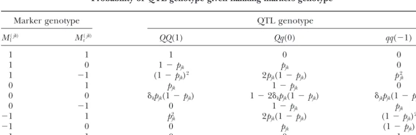
TABLE 2

Probability of QTL genotype given flanking markers genotype

Marker genotype QTL genotype

M(jk)

l M(rjk) QQ(1) Qq(0) qq(⫺1)

1 1 1 0 0

1 0 1⫺pjk pjk 0

1 ⫺1 (1⫺pjk)2 2pjk(1⫺pjk) p2jk

0 1 pjk 1⫺pjk 0

0 0 ␦kpjk(1⫺pjk) 1⫺2␦kpjk(1⫺pjk) ␦jkpjk(1⫺pjk)

0 ⫺1 0 1⫺pjk pjk

⫺1 1 p2

jk 2pjk(1⫺pjk) (1⫺pjk)2

⫺1 0 0 pjk (1⫺pjk)

⫺1 ⫺1 0 0 1

pjk⫽rjk/rM(_ljk)M_r(jk), ␦jk⫽r2M(_ljk)M_r(jk)/((1⫺rM_l(jk)M(_rjk))2⫹r2M(_ljk)M(_rjk)), where rjk is the recombination frequency

between markerM(jk)

l and QTLQin thejth individual andrM (jk)

l M

(jk)

r is the recombination frequency between

markersM(jk)

l andM

(jk)

(3)

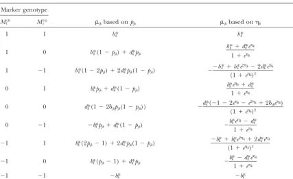
TABLE 3

␮˜jkconditional on flanking markers’ genotype, assuming complete interference

Marker genotype

M(k)

l M(rk) ␮˜jkbased onpjk ␮˜jkbased on␩k

1 1 b*k b*k

1 0 b*k(1⫺pjk)⫹d*kpjk

b*k ⫹d*ke␩k

1⫹e␩k

1 ⫺1 b*k(1⫺2pjk)⫹2d*kpjk(1⫺pjk) ⫺⫺

b*k ⫹b*ke2␩k⫺2d*ke␩k

(1⫹e␩k₎2

0 1 b*kpjk⫹d*k(1⫺pjk)

b*ke␩k⫹d*k

1⫹e␩k

0 0 d*k(1⫺2␦jkpjk(1⫺pjk)) ⫺

d*k(⫺1⫺2e␩k⫺e2␩k⫹2␦jke␩k)

(1⫹e␩k₎2

0 ⫺1 ⫺b*kpjk⫹d*k(1⫺pjk) ⫺

b*ke␩k⫺d*k

1⫹e␩k

⫺1 1 b*k(2pjk⫺1)⫹2d*kpjk(1⫺pjk)

⫺b*k ⫹b*ke2␩k⫹2d*ke␩k

(1⫹e␩k₎2

⫺1 0 b*k(pjk⫺1)⫹d*kpjk ⫺

b*k ⫺d*ke␩k

1⫹e␩k

⫺1 ⫺1 ⫺b*k ⫺b*k

In conclusion, provided we can specify the mean func- be dealt with below—and introduce the GEE approach tion␮(␥) and the covariance matrixV(␣), we can obtain using the familiar special case of normally distributed consistent estimates of the parameters of interest␥using traits. Denoting the phenotypic value of the kth trait GEE. We now derive a suitable mean and variance struc- in thejth individual byyjk, the corresponding random

ture for multivariate QTL mapping. variable by Yjk, and the random variable of the

unob-QTL mapping via GEE:Suppose we havenindividuals served QTL score byQjk, we assume the connection

be-from an F2population resulting from a cross between tween the phenotypic informationYijandQjkis given by

two inbred lines, with observations on m quantitative

Yjk⫽b*kQjk⫹ d*k1{Qjk⫽0}⫹xjk␤ ⫹ εjk, (5)

traits and on a number of codominant genetic markers for each individual. The markers are recorded as 1 and

whereb*k is the additive effect of the QTL that is to be

⫺1 for the homozygotes in the two parental lines and

mapped for thekth trait,d*k is the dominance effect of

0 for the heterozygotes. The same notation is also

ap-the QTL that is to be mapped for ap-the kth trait, Xj ⫽

plied for the unobserved QTL genotypes, with

homozy-(xt

j1, . . . ,xtjm)t 僆⺢m⫻p is the design matrix and xjk 僆

gotes coded as 1 and⫺1 and heterozygotes as 0. We

⺢1⫻p_,_k⫽_{1, . . . ,}_m_{is the design vector of other predictor}

assume that a marker map exists, although we show

variables for thejth individual,␤僆⺢p_{is the parameter}

below that uncertainty about intermarker

recombina-vector,1{.}is the indicator function, andεjkis the error

tion fractions can easily be accommodated.

term. Note thatXjmay include other markers fitted as

We now derive the mean and variance structure

re-cofactors, as is standard in univariate QTL mapping, to quired for our GEE model. We begin by considering

give an approximate multiple-QTL model. Alternatively, the estimation of location and effect for a single QTL

we can easily extend Equation 5 to include multiple for each trait—we consider how multiple QTL might

QTL for each trait by adding appropriate terms depen-dent on a second unobserved QTL score,Q⬘jk. For ease

TABLE 4 of explanation we omitted epistatic and pleiotropic ef-fects, but these can also easily be added to Equation 5. Locations and distributions of the QTL

Let the random variables representing the marker genotype of the left and right flanking markers in the Traitk Position Distribution ␪k φk b*k d*k

jth individual and thekth trait beM(jk)

l andM(rjk),

respec-1 3 Poisson 3.00 1.00 0.20 ⫺0.10

tively, and the realized values of these random variables 2 94 Binomial 0.00 1_⁄

10 0.30 0.15

bex(jk)

(4)

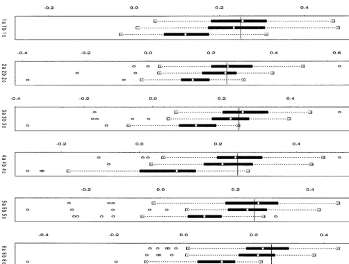
Figure1.—Simulation experiment. Comparison of simultaneous QTL-mapping methods for two nonnormal traits. The box plots for the estimates for the QTL location of the first trait and second trait are shown. The plots are described in Table 5.

we are allowing the marker interval containing the QTL genotype, the phenotypic distribution is a mixture of to be mapped for thekth trait to depend onk.Assume components corresponding to the unknown QTL geno-that the environmental random errors (εj1, . . . , εjm) type, we average out the unknown QTL genotypes to

have a multivariate normal distribution with mean zero get the conditional mean. Our approach can therefore and covariance matrix 兺(␣) 僆⺢m⫻m dependent on a be seen to be a generalization of the mean assumption of parameter vector␣僆⺢s_{: Errors are assumed}

indepen-the least-squares-based QTL-mapping methods (Haley dent across individuals, but correlated across traits. De- andKnott1992;Martı´nezandCurnow1992) to mul-noting the mean of Yij conditional on the flanking tivariate data.

marker information, M(jk)

l ⫽ x(ljk)and Mr(jk)⫽ x(rjk), and Now consider the second moment assumption. To

other potentially genetically determined predictor vari- simplify notation, we initially derive the “working” vari-ables,Xjk⫽ xjk, by ance matrix under the simplest possible model. We

as-sume that there is no gene-environment or genetic inter-␮jk⫽E(Yjk|Ml(jk)⫽ x(ljk),M(rjk)⫽ xr(jk),Xjk⫽xjk), (6)

action and that the predictor variablesXjkare independent

we formulate our first moment assumption as _{of the flanking marker score. Then the variance of} _Y_jk conditional on the flanking marker information can be

␮jk⫽E(b*kQjk⫹d*k1{_Qjk⫽0}|M(ljk)⫽x(ljk),M(rjk)⫽x(rjk))⫹xjk␤i.

written as Note the distinction between this and the

full-likeli-hood approach ofJiangandZeng(1995): Rather than _Var_ 

Yj1|M(lj1) ⫽ x(lj1),Mr(j1) ⫽x(rj1),Xj1 ⫽xj1

⯗

Yjm|M(ljm)⫽x(ljm),Mr(jm)⫽x(rjm),Xjm⫽xjm

(5)

Figure1.—Continued.

⫽Var

  

b*1Qj1⫹d*11{_{Q j}₁⫽0}|M(lj1) ⫽x(lj1),M(rj1)⫽x(rj1),Xj1 ⫽xj1

⯗

bm*Qjm⫹d*m1{_{Q jm}⫽0}|M(ljm)⫽x(ljm),Mr(jm)⫽x(rjm),Xjm⫽xjm

 

 Var

  

Yj1|M(lj1) ⫽x(lj1),Mr(j1)⫽x(rj1),Xj1 ⫽xj1 ⯗

Yjm|M(ljm)⫽x(ljm),Mr(jm)⫽x(rjm),Xjm⫽xjm

  ≈Var

   εj1

εjm  

. (8)

Again this is the variance assumption taken by the

least-⫹Var

   εj1

εjm  

. (7) _{squares-based QTL mapping methods (Haley} _and

Knott1992;Martı´nezandCurnow1992). The limita-This is the well-known decomposition of the phenotypic

tions of variance assumption (8), which are primarily variance Var(Yjk | M(ljk) ⫽ x(ljk), M(rjk) ⫽ x(rjk)) into the _{due to ignoring variance due to the segregation of QTL}

genetic variance due to segregation of the QTL within _{within marker classes, have been discussed in detail by} marker classes and the environmental variance Var(εjk) _Xu _{(1995) and} _Kao _{(2000). However, recall that, in}

(6)

Figure2.—Simulation experiment. Comparison of simultaneous QTL-mapping methods for two nonnormal traits. The box plots for the estimates for additive effect and for the dominance effect of the first trait are shown. The plots are described in Table 5.

tion and multiple QTL, the GEE approach based on such that we can transform the mean ofYjk, conditional

on the explanatory variables, to be a linear function variance assumption (8) will provide consistent

esti-mates for all mean parameters and correct standard of those explanatory variables. Although there are no general rules of thumb for the choice of the link func-errors for these estimates. Although a misspecified

vari-ance assumption might have an influence on the effi- tion, it is usually suggested to choose the link function so that the data, after being transformed by the link ciency of the estimates, the loss of efficiency is usually

function, look as “normal” as possible (Johnson and slight, even if the working variance matrix (8) is

substan-Wichern1992). For some typical traits,e.g., continuous tially misspecified (LiangandZeger1986;Lianget al.

phenotype, counts, proportions, Table 1 lists some ap-1992). The use of a GEE approach thus largely

compen-propriate link functions that are commonly used for sates for the limitations of variance assumption (8).

GEE models (McCullaghandNelder 1989). We now extend this model to deal with nonnormal

The variance matrix is then constructed on the basis traits. This is easily done by applying a link function

of the link function. We assume that a correlation matrix hk(␮jk) to the conditional mean ofYjk(McCullaghand

R(␣) 僆⺢m⫻m is given that depends upon correlation Nelder1989), which gives the following mean

assump-parameter vector␣僆⺢q_{that can be interpreted as the}

tion:

environmental correlation. When more sophisticated hk(␮jk)⫽E(b*kQjk⫹d*k1{_{Q jk}⫽0}|Ml(jk)⫽x(ljk)Mr(jk)⫽x(rjk))

variance structures are modeled ␣ might also contain

⫹xjk␤. (9)

(7)

trix for nonnormal traits by rescaling the correlation are based on a graphical data analysis where one tries to investigate functional relationship between the variance matrixR(␣) with the corresponding variance functions

and dispersion parameters;i.e., and the mean. Typical choices for dispersion parame-ters and variance functions are listed in Table 1 (McCul-laghandNelder1989).

Vj⫽ Var

冢

Yj

兩

冢

M(j1)

l ⫽ x(lj1),M(rj1) ⫽x(rj1),Xj1 ⫽ xj1

⯗ M(jm)

l ⫽x(ljm),Mr(jm)⫽x(rjm),Xjm⫽xjm

冣冣

Calculation of the conditional means:Here we show how

to calculate the expectations given marker genotypes ⫽ ⌽1

2A

1/2

j R(␣)A1/2j ⌽1/2, (10) _{required in}␮

jk; that is, we calculate

␮˜jk⫽ b*k

兺

1

qjk⫽⫺1

qjkp(qjk|M(ljk)⫽xl(jk),M(rjk)⫽x(rjk))

where Aj ⫽ diag(V1(␮j1), . . . , Vm(␮jm)) is a diagonal

matrix of variance functions and⌽ ⫽diag(φ1, . . . ,φm) _⫹

d*kp(0|M(ljk)⫽xl(jk),Mr(jk)⫽x(rjk)). (11)

is a diagonal matrix of the dispersion parameters for

themtraits. The variance functions and dispersion pa- The conditional probability p(qjk|M(ljk)⫽ x(ljk),M(rjk)⫽

rameters must also be specified by the scientist. They x(jk)

r ) is easily done given a model for recombination.

(8)

Figure3.—Simulation experiment. Comparison of simultaneous QTL-mapping methods for two nonnormal traits. The box plots for the estimates for the additive effect and for the dominance effect of the second trait are shown. The plots are described in Table 5.

JiangandZeng(1995) assumed complete interference the conditional mean␮jkin Table 3 is influenced only

within marker intervals (i.e., no double recombinants) by the marker interval length for marker score (0, 0). in the multivariate approach. Either assumption is easily It can be shown that when␩kis estimated instead ofrjk,

incorporated into the GEE approach. For simplicity, we the conditional mean␮˜jkin Table 3 is virtually

indepen-consider here only the complete interference case. dent of the marker interval lengthrM(_ljk)M(_rjk)(appendix).

Following the complete interference assumption of The GEE approach with parameterization (12) is there-Jiang and Zeng (1995), expressions for p(qjk|M(lk)⫽ fore also robust against misspecification of the

marker-x(jk)

l ,M(rk)⫽xr(jk)) and hence for␮jkcan be easily derived; interval length, which allows QTL analysis to be

per-these are given in Tables 2 and 3. Further, when we formed even if the intermarker distances are unknown, reparameterize the recombination fraction between the provided the marker ordering is known reliably. This left-flanking marker and the QTL by is potentially valuable since StringhamandBoehnke (2001) reported that misspecification of the marker rjk⫽

exp(␩k)

1⫹exp(␩k)

rM(_ljk)M(_rjk), (12) map can have a substantial effect on likelihood analysis

for human data. For parameterization (12) the analyti-cal expressions for␮˜jkare also shown in Table 3. Note

where rM(_ljk)M(_rjk) is the recombination fraction between

that when the marker-interval lengths are known param-the flanking markers, parameterpjkin Table 2 becomes

(9)

parameterization that the estimate for the QTL location

_兺

n

j⫽1

DT

j Vj(␮j,␣)⫺(Yj⫺ ␮j(␥ˆ))⫽ 0. (13)

is range preserving; i.e., the estimated QTL position

must lie between the flanking markers, which give much _Here_V

j(␮,␣) is the working variance described above

improved numerical properties. _and_␮_j_⫽₍_␮_j₁_{, . . . ,}_␮_jm_{), where}_␮_jk_{is the expected value} Parameterization (12) also gives robustness to varia- of the kth trait for the jth individual, which is easily calculated under either the complete interference as-tion in map lengths between individuals, for example,

sumption or the no-interference assumption: because of sex effects, although in practice sex-averaged

recombination rates usually give satisfactory results with _␮

jk⫽ E(Yjk)⫽h⫺j 1

共

␮˜jk⫹

兺

i

xki␤i

兲

. (14)

most methods. Finally, note that these results also hold for the no-interference case.

Equation 3 also involves the matrix of derivatives of

Parameter estimation: Parameter estimation is

per-each individual’s phenotypic means,Dj, which is given by

formed using a simple extension of the standard GEE approach described byLiangandZeger (1986). The

details, which are by their nature rather technical, can Dj⫽diag

冢

⳵h⫺1 1 (␪)

⳵␪

兩

_␪⫽h

1(␮j1)

, . . . ,⳵h

⫺1 m (␪)

⳵␪

兩

_␪⫽h

1(␮jm)

冣

(X˜j|Xj)

be found inLange(2000); here we sketch the key steps of the estimation procedure. Recall from Equation 3

(10)

TABLE 5

Description of plots for Figures 1–3: notation for the combinations of QTL-mapping methods and environmental

correlations







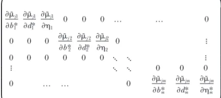
⳵␮˜j1

⳵b*1

⳵␮˜j1

⳵d*1

⳵␮˜j1

⳵␩1

0 0 0 … … 0

0 0 0 ⳵␮˜j2

⳵b*2

⳵␮˜j2

⳵d*2

⳵␮˜j2

⳵␩2

0 ⯗

0 0 0 0 0 0 _⯗ _⯗ ⯗

⯗ _⯗ _⯗ 0 0 0

0 … … 0 ⳵␮˜jm

⳵b*m ⳵␮˜jm

⳵d*m ⳵␮˜jm ⳵␩*m







. Environmental correlation

Method ⫺0.6 ⫺0.3 0.0 0.3 0.6 0.9

I 1a 2a 3a 4a 5a 6a

II 1b 2b 3b 4b 5b 6b

III 1c 2c 3c 4c 5c 6c

The partial derivatives in matrixX˜jare easily computed

Method I, GEE approach using link functions and untrans-from the expressions given in Table 2.

formed data; method II, transforming the data to normality Equation 3 can then be solved by a two-step procedure

and using the GEE approach under normality assumption; that iterates between an updating step for the mean

method III, ignoring the nonnormality of the data and using parameter estimates, on the basis of the current values _{the GEE approach under normality assumption.}

of the variance parameters, and an updating step for _{The solid lines in the box plots in Figures 2–4 show the} the variance parameters, on the basis of the current _{true QTL positions. Box plots show the median, 25th, and} estimates of the mean parameters. In the first step, the 75th percentiles, together with whiskers showing the range of estimates of the mean parameter vector ␥ ⫽ (b*1,d*1, the data provided it is ⬍1.5 times the interquartile range;

points beyond this are marked as outliers. ␩1, . . . ,b*m,d*m,␩m,␤T) are updated by

␥ˆt⫹1⫽ ␥ˆt

types relies on searching the genome for putative QTL

⫹

冦

_兺

n

j⫽1

DT

j(␥ˆt)V⫺(␥ˆt,␣ˆt)Dj(␥ˆt)

冧

⫺

locations, which give maxima in the likelihood or min-ima in the residual sum of squares, according to the

⫻

冦

_兺

n

j⫽1

DT

j(␥ˆt)V⫺(␥ˆt,␣ˆ)

共

yj⫺(␮j1(␥ˆt), . . . ,␮jm(␥ˆt))T)

冧

approach chosen; approximate multiple-QTL models (15) _{are usually fitted by selecting a set of markers, usually} with yj⫽ (yj1, . . . ,yjm)T. Then in the second step new _{via a model selection criterion such as AIC, to include}

estimates for the variance parameters are calculated as _{as cofactors when scanning the genome. The evidence} follows. We compute the residuals bysjk⫽ (yjk ⫺ ␮ˆjk)/ for a QTL at any location can then be assessed.

(Vk(␮ˆjk))0.5, estimate the dispersion parameters byφˆk⫽ _{In the above we have shown how QTL location and}

1/(n⫺ 3m⫺p)

兺

n

j⫽1s2jk, compute the standardized re- _{effect size can be estimated for a given set of marker}

siduals bysˆ⬘jk⫽ rjk/

√

φˆk, and estimate the correlation pa- intervals using our GEE approach, but we have not yet

rameter vector␣by moment-based estimators using the _{considered how models for different marker intervals} standardized residuals sˆ⬘jk. This two-step procedure is can be compared. It is not obvious how to do this in the

then repeated until parameter estimates converge. _{GEE framework: One of the strengths of the approach is} Note that this gives estimates of all parameters, includ- _{that we need not specify a full probability model for} ing the QTL locations ␩, conditional on the specified _{the data, so we have no likelihood to use in model} flanking markers. Refitting with QTL at a number of _{comparison. The quasi-likelihood defined above can} points within the specified marker intervals to produce _{sometimes be used to play a similar role, but we have} a residual sum of squares (RSS) surface as is usual in _{already commented that quasi-likelihood is not available} least-squares-base QTL mapping is not required. _{for our QTL model.}

An attractive property of this procedure is that under _{A natural alternative to quasi-likelihood is the} general-mild conditions, notably that the moment-based estima- _{ized Pearson chi-square statistic}

tors␣ˆ andφˆ1, . . .,φˆmare consistent, the GEE estimate␥ˆG

is also consistent and asymptotically multivariate normal,

d*⫽

兺

n

j⫽1

(yj⫺␮j)TV⫺j (␮j)(yj⫺ ␮j). (16)

i.e.,n1/2 (␥ˆG ⫺ ␥) is asymptotically multivariate normal

with mean zero and covariance matrixVGgiven by

Loosely, d* is a weighted sum of residuals with the

VG⫽lim

n→∞n

冢冢

兺

n

j⫽1

DT jV⫺jDj

冣

⫺

冢

兺

n

j⫽1

DT_V⫺

jCov(Yj)V⫺jDj

冣冢

兺

n

j⫽1

DT jV⫺j Dj

冣

⫺

冣

weights calculated from the variance matrix calculated at the parameter estimates. Other statistics could be utilized here, butd* is attractive since it fulfills all the with Yj⫽(Yj1, . . . ,Yjm)T.

requirements of a goodness-of-fit statistic (Coxand Hink-It is important to note that the validity of this result

ley 1974) and has attractive theoretical properties does not depend on the correct specification of the

(Lange2000);i.e.,d* is a second-order approximation variance assumption. Regardless of the degree of

mis-of the true quasi-deviance function. specification, the mean parameter estimates are always

Models can now be compared just as for the least-consistent and the standard errors provided are correct.

(11)

2000) by replacing the usual RSS byd*. However, as with data. This is of interest sinceVisscheret al.(1996a,b) the least-squares-based methods, significance thresholds found that assuming normality often works well for should be obtained by permutation (Doerge and univariate binary traits.

Churchill1996) or by use of the parametric bootstrap,

A relatively simple experiment is sufficient to compare rather than by reliance on asymptotic results.

Further-these methods. We simulate a single chromosome with more, analogues of the standard model selection criteria

16 uniformly distributed markers; the marker interval used for linear models can then be defined by replacing

length is 10 cM, giving a total length of 150 cM. Data the usual residual sum of squares byd*. For example,

are simulated using the following mean assumption: we can define the Akaike information criterion (AIC)

for a given GEE model to be

qjk⫽1: E(Yjk)⫽hk⫺1(␪k⫹b*k)

qjk⫽0: E(Yjk)⫽ hk⫺1(␪k⫹ d*k)

AIC ⫽d*⫹2number of predictor variables

sample size . qjk⫽ ⫺1:E(Yjk)⫽hk⫺1(␪k⫺ b*k). (17)

Alternatively, the AIC-value approximation for general- _{Two traits are simulated, both representing count data,} ized estimating equations byPan(2001) may be applied _{with the first generated by a Poisson distribution and}

here. _{the second from a binomial distribution on 10 trials.}

Any of the standard approaches for QTL analysis can _{The parameter values used can be found in Table 4.} now be implemented. For instance, to reproduce the _{By standard theory, the appropriate transformations to} original interval-mapping approach of Lander and _{normality for use in method II are thus ln (·) for the} Botstein(1988) for a single trait using GEE we would _{first trait and ln{(·/10)/(1}_⫺_{·/10)} for the second trait.} simply fit a single-QTL model for each interval in turn _{The simulation was conducted for environmental} corre-using the procedure outlined above. This provides esti- _{lation values}

mates of QTL location and effect, together with a value

ofd*, corresponding to a model with a single QTL in ⫺0.6,⫺0.3, 0.0, 0.3, 0.6, and 0.9, the interval currently under consideration. The interval

with sample size 600 in each case and 200 replicates. with the smallest value ofd* is then selected, and the

Results are summarized using box plots displaying the corresponding estimates of QTL location and effect are

median, 25th percentile, 75th percentile, and the range recorded. The QTL will be declared significant ifd* is

of the estimated location; and additive and dominance below an appropriate threshold, determined by

permu-effects over the 200 replicates. The results are in Figures tation or simulation as in the least-squares-based

ap-1–3 and Table 5. It is immediately obvious that the proaches.

efficiency of the methods differs substantially. Method Equivalents to composite interval mapping (Zeng

I gives more efficient estimates of QTL location and 1994) or multiple-QTL mapping (Jansen 1994) can

additive effect, with methods II and III giving estimates be produced by including markers, usually selected by

of additive effect with considerable bias. Thus even mar-stepwise variable selection using AIC or similar criteria,

ginal transformation to normality followed by an analy-as cofactors to control for the presence of QTL outside

sis assuming multivariate normality (method II), al-the interval currently under consideration. It is also of

though an improvement on use of the untransformed course possible to fit models containing QTL in several

data, is less efficient than the pure GEE approach. Nor-intervals simultaneously, by adding the appropriate terms

mal theory alone is clearly not sufficient to cope with to the models described above. Tests to dissect the genetic

architecture of multiple traits can be defined as inKnott nonnormally distributed traits.

andHaley(2000), withd* replacing the RSS. In particu- The poor performance of method III above shows lar, a test of a single pleiotropic QTL against linked QTL, that the good performance of method III for univariate each affecting a single trait, is produced by comparing binary traits observed byVisscheret al.(1996a,b) does thed* values for the relevant models. not generalize. We can explain the good performance of method III for univariate binary traits by noting that RESULTS _{for univariate binary data the score equation of the GEE}

model for method I is given by

Simultaneous QTL mapping for two nonnormally dis-tributed traits:Here we compare the GEE approach to

two alternatives that do not explicitly model the nonnor- 0⫽

兺

n

j⫽1

冦

⳵h⫺1₍␪₎

⳵␪

兩

␪⫽h(␮_j)(X˜j|Xj)

冧

φ⫺1V⫺(␮j)(Yj⫺ ␮j(␤))

mality of the data. The methods used were as follows:

⫽

_兺

n

j⫽1

兵

V(␮j)(X˜j|Xj)

其

φ⫺1V⫺(␮j)(Yj⫺ ␮j(␤))

Method I: The GEE approach described above. Method II: The data are transformed to normality and

⫽φ⫺1

兺

n

j⫽1

(X˜j|Xj)(Yj⫺h⫺1)

兵

(X˜j|Xj)␤

其

) (18)

the appropriate GEE for multivariate normal re-sponses is used (i.e., identity link function, etc.).

with␮j(␤) = (␮j1(␤), . . . ,␮jm(␤)). Since the inverse link

Method III: The GEE method appropriate for

(12)

binary data is a rather “linear” function that can locally could be obtained by bootstrapping as in Visscher et al.(1996a,b). However, multivariate QTL mapping by its be approximated very well by its first-order Taylor

ap-proximation, Equation 18 can be approximated by nature becomes increasingly computationally demanding as the number of responses increases, so these

com-φ⫺1

兺

n

j⫽1

(X˜j|Xj)(Yj ⫺

兵

(X˜j|Xj)␤˜

其

), (19) puter-intensive techniques may be at present limited to

relatively small numbers of responses. These are in any which is the estimating equation of method III. Thus case the situation where application of multivariate tech-for univariate binary data methods I and III give almost niques seems most likely, but less computationally de-equivalent estimating equations, but this will not be true manding solutions to the threshold/confidence interval

in general. problems would nonetheless be useful, and this subject

Note that this argument applies also to univariate deserves further study. Finally we note that the GEE likelihood-based methods, since in the univariate case approach developed here has obvious applications to the likelihood score and GEE score are identical. marker-assisted selection for multivariate nonnormal

traits. We hope to investigate this elsewhere. DISCUSSION

We thank Dr. Zhao-Bang Zeng and the unknown referee for their

We have introduced a method to allow the simultane- constructive comments on an earlier draft of this article. This research was supported by grant MH59532 of The National Institutes of Health.

ous mapping of QTL for several nonnormal traits. Ex-plicitly multivariate analyses of this sort have several advantages over the alternative approach based around

a number of single-trait analyses, notably the ease of LITERATURE CITED

interpretation of results and the increased efficiency of _{Cox, D. R}_{., and}_{D. V. Hinkley}_{, 1974} _{Theoretical Statistics.}_{Chapman &}

Hall, London/New York.

multivariate analyses (JiangandZeng1995;Korolet

Dempster, A. P., N. M. LairdandD. B. Rubin, 1977 Maximum

al. 1995). It is also possible to test for pleiotropy,

al-likelihood from incomplete data via the EM-algorithm. J. R. Stat.

though in practice it is very difficult to distinguish be- _Soc._39:_1–38.

Diggle, P. J., K.-Y. LiangandS. L. Zeger, 1996 Analysis of

Longitudi-tween several linked QTL, each affecting a single trait,

nal Data.(Oxford Statistical Science Series). Oxford University

and a single QTL with pleiotropic effects.

Press, London/New York/Oxford.

However, full probability models for multivariate non- _{Doerge, R. W}_{., and}_{G. A. Churchill}_{, 1996} _{Permutation tests for}

multiple loci affecting a quantitative character. Genetics142: normal responses are very difficult to specify, and it is

285–294.

therefore tempting to either ignore the nonnormality

Falconer, D. S., andT. F. C. Mackay, 1997 Introduction to

Quantita-or marginally transfQuantita-orm the data to nQuantita-ormality and then _{tive Genetics.}_{Longman, New York.}

Hackett, C. A., andJ. I. Weller, 1997 Genetic mapping of

quantita-assume multivariate normality in analysis. As the

simula-tive trait loci for traits with ordinal distributions. Biometrics51: tion experiment shows, doing this can give poor results.

1252–1263.

Instead we avoided the difficulties of full-likelihood _{Haley, C. S}_{., and}_{S. A. Knott}_{, 1992} _{A simple regression method}

for mapping quantitative trait loci in line crosses using flanking

methods by adopting a semiparametric approach based

markers. Heredity69:315–324.

on GEE. The key advantages are the avoidance of

distri-Haley, C. S., andS. A. Knott, 2000 Multitrait least squares for

butional assumptions, the ease and flexibility of model _{quantitative trait loci detection. Genetics}_158:_899–911.

Henshall, J. M., andM. E. Goddard, 1999 Multiple-trait mapping

specification [for example, the model presented here

of quantitative trait loci after selective genotyping using logistic

could be easily extended to incorporate factors such as

regression. Genetics151:885–894.

epistasis or parent of origin (imprinting) effects], and the _{Heyde, C}_{., 1997} _{Quasi-likelihood and Its Application.}_{Springer Series}

in Statistics, Berlin/Heidelberg, Germany/New York.

robustness of estimates of QTL parameters to

misspeci-Jansen, R. C., 1994 High resolution of quantitative traits into

multi-fication of the underlying variance structure. We have

ple loci via interval mapping. Genetics136:1447–1455.

also shown that a simple reparameterization leads to a _{Jiang, C}_{., and} _{Z-B. Zeng}_{, 1995} _{Multiple trait analysis of genetic}

mapping for quantitative trait loci. Genetics140:1111–1127.

method for which the intermarker distances need not

Johnson, R. A., andD. W. Wichern, 1992 Applied Multivariate

Statisti-be known.

cal Analysis.Prentice-Hall International, Englewood Cliffs, NJ.

GEE methods are often almost as efficient as full- _{Kao, C.-H}_{., 2000} _{On the differences between maximum likelihood}

and regression interval mapping in the analysis of quantitative

likelihood approaches using the correct probability

trait loci. Genetics156:855–865.

model, while being more robust. Nonetheless, it would

Knott, S. A., and C. S. Haley, 2000 Multitrait least squares for

be interesting to develop full-likelihood approaches and _{quantitative trait loci detection. Genetics}_158:_899–911.

Korol, A. B., Y. T. RoninandV. M. Kirzhner, 1995 Interval

map-to compare these with the GEE approach. This should

ping of quantitative trait loci employing correlated trait

com-be possible for at least some special cases, possibly using

plexes. Genetics140:1137–1147.

generalized linear mixed models or hierarchical models _{Lander, E. S}_{., and}_{D. Botstein}_{, 1988} _{Mapping Mendelian factors}

underlying quantitative traits using RFLP linkage maps. Genetics

implemented in a Bayesian framework via the Markov

121:185–199.

chain Monte Carlo method. However, such an approach

Lange, C., 2000 Generalized estimating equation methods in

statisti-will be extremely computationally demanding, even for _{cal genetics. Ph.D. Thesis, University of Reading, Reading, UK.}

Liang, K.-Y., andS. L. Zeger, 1986 Longitudinal data analysis using

relatively small numbers of traits.

generalized linear models. Biometrika73(1): 13–22.

Significance thresholds for the GEE approach can

Liang, K.-Y., S. L. ZegerandB. Qaqish, 1992 Multivariate

regres-be calculated by the usual permutation or simulation _{sion analyses for categorical data. J. R. Stat. Soc. B}₅₄_{(1): 3–40.}

Martı´nez, O., andR. N. Curnow, 1992 Estimating the locations

(13)

and the sizes of the effects of quantitative trait loci using flanking markers. Theor. Appl. Genet.85:480–488.

McCullagh, P.,andJ. A. Nelder, 1989 Generalized Linear Models,

Ed. 2. Chapman & Hall, London/New York.

Pan, W., 2001 Akaike’s information criterion in generalized estimat-ing equations. Biometrics57:120–125.

Stringham, H. M.,andM. Boehnke, 2001 Lod scores for gene mapping in the presence of marker map uncertainty. Genet. Epidemiol.21:31–39.

Visscher, P. M., C. S. Haleyand S. A. Knott, 1996a Mapping QTLs for binary traits in backcross and F2 generation. Genet. Res.68:55–63.

Visscher, P. M., R. ThompsonandC. S. Haley, 1996b Confidence intervals in QTL mapping by bootstrapping. Genetics140:1013– 1020.

Xu, S.,1995 Letter to the editor: A comment on the simple regres-sion method for interval mapping. Genetics141:1657–1659.

Zeng, Z-B., 1994 Precision mapping of quantitative trait loci. Genet-ics136:1457–1468.

Communicating editor:Z-B. Zeng

APPENDIX

Robustness of reparameterization (12):We can inves-tigate the influence of the marker interval length rM(_ljk)M(_ljk)on the component of the conditional mean for

marker class (0, 0) that depends onrM(_ljk)M(_ljk)by plotting

f(␲,x)⫽{1⫺ 2·␦jkpjk(1⫺ pjk)} (20)

against x, the marker interval width in centimorgans, and␲, the relative location of the QTL. This is shown as the top surface in Figure A1. The bottom surface

presents the relative frequency of marker class (0, 0) FigureA1.—Relative influence of the marker-interval size on the mean equation for the marker-score (0, 0). The top dependent on the marker interval width in

centi-plane shows the relative dependency of the mean equation morgans; Haldane’s mapping function has been used to

for marker score (0, 0) as a function of the marker interval convert distances in centimorgans into recombination _{length and the relative QTL position, assuming complete} in-fractions. We see that the conditional mean is only _{terference. The bottom plane shows the frequency of marker} weakly dependent onx and that marker-class (0, 0) is score (0, 0) as a function of the marker interval length and