Sensory Relevance Models

Portland State University Portland State University

PDXScholar

PDXScholar

Dissertations and Theses Dissertations and Theses

Summer 8-8-2019

Sensory Relevance Models

Sensory Relevance Models

Portland State University

Follow this and additional works at: https://pdxscholar.library.pdx.edu/open_access_etds

Part of the Computer Sciences Commons

Let us know how access to this document benefits you.

Recommended Citation Recommended Citation

Woods, Walt, "Sensory Relevance Models" (2019). Dissertations and Theses. Paper 5123.

10.15760/etd.7002

Sensory Relevance Models

by Walt Woods

A dissertation submitted in partial fulfillment of the requirements for the degree of

Doctor of Philosophy in

Electrical and Computer Engineering

Dissertation Committee: Christof Teuscher, Chair

Dan Hammerstrom Gerardo Lafferriere

Bart Massey

Portland State University 2019

c

Abstract

This dissertation concerns methods for improving the reliability and quality of explanations for decisions based onNeural Networks (NNs). NNs are increasingly part of state-of-the-art solutions for a broad range of fields, including biomedical, logistics, user-recommendation engines, defense, and self-driving vehicles. While NNs form the backbone of these solutions, they are often viewed as “black box” solutions, meaning the only output offered is a final decision, with no insight into how or why that particular decision was made. For high-stakes fields, such as biomedical, where lives are at risk, it is often more important to be able to explain a decision such that the underlying assumptions might be verified.

Prior methods of explaining NN decisions from images have been proposed, and fall into one of two categories: post-hoc analyses and attention networks. Post-hoc analyses, such as Grad-CAM, look at gradient information within the network to identify which regions of an image had the greatest effect on the final decision. Attention networks consist of structural changes to the network, which produce a mask through which the image is filtered before subsequent processing. The result is a heatmap highlighting regions which have the greatest effect on the final decision. This dissertation identifies two flaws with these approaches. First, these methods of explanation change wildly when the network is exposed to adversarial examples. When an imperceptible change to the input results in a significant change in the explanation, how reliable is the explanation? Second, these methods all produce a heatmap, which arguably does not have the definition required to truly understand which features are important. An algorithm that can draw a circle around a cat does not necessarily know that it is looking at a cat; it only recognizes the existence of a salient object.

To address these flaws, this dissertation explores Sensory Relevance Models

(SRMs), methods of explanation which utilize the full richness of the sensory do-main. Initially motivated by a study of sparsity, several incarnations of SRMs were evaluated for their ability to resist adversarial examples and provide a more informative explanation than a heatmap.

The first SRM formulation resulted from a study of network bisections, where NNs were split into a pre-processing step (the SRM) and a classifying step. The result of the pre-processing step would be made very sparse before being passed to the classifier. Visualizing the sparse, intermediate computation would potentially have yielded a heatmap-like explanation, with the potential for more textured ex-planations being formed off of the myriad features comprising each spatial location of the SRM’s output. Two methods of achieving network bisection using auxiliary losses were devised, and both were successful in generating a sparse, intermediate representation which could be interpreted by a human observer. However, even a network bisection SRM which used only 26 % of the input image did not result in decreased adversarial attack magnitude. Without solving the adversarial attack issue, any explanation based on the network bisection SRM would be as fragile as previously proposed methods.

That led to the theory of Adversarial Explanations (AE). Rather than trying to produce an explanation in spite of adversarial examples, it made sense to work with them. For images, adversarial examples result in full-color, high-definition output. If they could be leveraged for explanations, they would solve both of the flaws identified with previous explanation techniques. Through new mathe-matical techniques, such as a stochastic Lipschitz constraint, and designing new mechanisms for NNs, such as the Half-Huber Rectified Linear Unit, AE were very

successful. On ILSVRC 2012, a dataset of 1,281,167 images of size 224×224 com-prising 1,000 different classes, the techniques for AE resulted in NNs 2.4× more resistant to adversarial attacks than the previous state-of-the-art, while retain-ing the same accuracy on clean data and usretain-ing a smaller network. Explanations generated using AE possessed very discernible features, with a more obvious in-terpretation when compared to heatmap-based explanations. As AE works with the non-linearities of NNs rather than against them, the explanations are relevant for a much larger neighborhood of inputs. Furthermore, it was demonstrated that the new adversarial examples produced by AE could be annotated and fed back into the training process, yielding further improved adversarial resistance through a Human-In-The-Loop pipeline.

Altogether, this dissertation demonstrates significant advancements in the field of machine learning, particularly for explaining the decisions of NNs. At the time of publication, AE is an unparalleled technique, producing more reliable, higher-quality explanations for image classification decisions than were previously avail-able. The modifications presented also demonstrate ways in which adversarial attacks might be mitigated, improving the security of NNs. It is my hope that this work provides a basis for future work in the realms of both adversarial resistance and explainable NNs, making algorithms more reliable for industry fields where accountability matters, such as biomedical or autonomous vehicles.

Acknowledgements

I am very grateful for the support and advice of my advisor, Christof Teuscher. Thank you to Jack H. Chen, Mohammad Taha, Kelsey Scharnhorst, Patrick Sheri-dan, and Jens B¨urger for helpful discussions and collaborations which contributed to this work. Thank you to A. Madry (from [41, 63]) and J. Cohen (from [11]) for helpful discussions and clarifications about their work. I would also like to thank FuR for assisting in the collection of photos used in examples throughout this work. This work was supported in part by the National Science Foundation under award # 1028378 and by the Defense Advanced Research Projects Agency (DARPA) under award # HR0011-13-2-0015. The views expressed are those of the author(s) and do not reflect the official policy or position of the Department of Defense or the U.S. Government.

Table of Contents

Abstract i

Acknowledgements iv

Table of Contents v

List of Tables viii

List of Figures ix Glossary xix 1 Introduction 1 1.1 Contributions . . . 8 1.1.1 Primary Contributions . . . 8 1.1.2 Auxiliary Contributions . . . 10

2 Locally Competitive Algorithm 13

2.1 LCA . . . 13 2.2 LCA and Deep Learning . . . 14 2.3 Supervised LCA . . . 15 2.4 Extending the Supervised LCA to SRMs via Network Bisection . . 18

3 Sensory Relevance Models via Network Bisection(s) 21

3.1 Related Work . . . 22 3.2 Theory . . . 24

3.2.1 Why Bisection? . . . 25

3.2.2 Required Traits . . . 28

3.3 Implementations and Results . . . 32

3.3.1 Activity Adjustment . . . 32

3.3.2 Gradient Integration Method . . . 39

3.4 Discussion . . . 46

4 Sensory Relevance Models via Adversarial Explanations 49 4.1 Related Work . . . 51 4.1.1 Adversarial Attacks . . . 51 4.1.2 Explanation Methods . . . 56 4.1.3 Human-in-the-Loop (HITL) . . . 59 4.1.4 Lipschitz Continuity . . . 61 4.2 Methods . . . 62

4.2.1 Adversarial Attack Generation and Evaluation . . . 63

4.2.2 Defense via Lipschitz Continuity . . . 69

4.2.3 Gradient Minimization as Weight Regularization . . . 73

4.2.4 Half-Huber Rectified Linear Unit (HHReLU) . . . 74

4.2.5 Output Zeroing . . . 75

4.2.6 Adaptiveψ . . . 77

4.2.7 Adversarial and Noisy Training . . . 77

4.2.8 Human-in-the-Loop (HITL) . . . 79

4.2.9 Architectures and Datasets . . . 80

4.2.10 Code Availability . . . 84

4.3 Results . . . 84

4.3.2 ImageNet Experiments . . . 104

4.3.3 COCO Experiments . . . 107

4.4 Combination with Network Bisection SRMs . . . 107

4.5 Oregon Health & Science University MEP-LINCS Report . . . 109

4.6 Discussion . . . 109

5 Conclusion 112 References 116 A Appendix Selected Papers 127 A.1 Adversarial Explanations for Understanding Image Classification Decisions and Improved Neural Network Robustness . . . 127

A.2 Fast and Accurate Sparse Coding of Visual Stimuli with a Simple, Ultra-Low-Energy Spiking Architecture . . . 128

List of Tables

4.1 Effect of Modifications on CIFAR-10 . . . 93

4.2 Effect of Modifications on CIFAR-10, Part II . . . 94

4.3 Effect of Adaptiveness on CIFAR-10 . . . 95

4.4 Effect of Adaptiveness on CIFAR-10, Part II . . . 96

List of Figures

1.1 Reproduction of Figure 3 from [28]. They proposed a very com-pelling, multi-level attention scheme which highlights salient objects wonderfully on the CIFAR-10 dataset. Furthermore, their scheme shows how the network’s attention is distributed at multiple levels within the network. Nonetheless, these highlights beg the question: within the regions marked salient, what qualities actually affect the network’s output? . . . 3 1.2 State-of-the-art methods of explaining an NN’s decision based on

some input (a) rely on the generation of some heatmap (b), gen-erated here via Grad-CAM [58]. In cases where the object’s shape is non-discriminatory, this provides little insight into the decision. Adversarial examples produce much richer output, and can be lever-aged to accentuate the NN’s decision (c), making salient features clearly visible when compared with the original image. Alterna-tively, some desired output may be encouraged to demonstrate fea-tures salient to that desired output (d). This technique also demon-strates training deficiencies - clearly, the COCO dataset contains few images of burgers from a top-down perspective, and a pile of ingredients is a strong indicator of sandwich-ness. Unless otherwise specified, all images in this paper were taken by the authors to avoid copyright issues. . . 6

2.1 Supervised extension to the LCA vs its original, unsupervised for-mulation. . . 17 3.1 SRMs via network bisection sought to provide an intermediate,

com-pressed representation of input signals that would be useful for human-in-the-loop debugging of data processing algorithms. . . 25 3.2 Network bisection SRMs require a high level of sparsity, which may

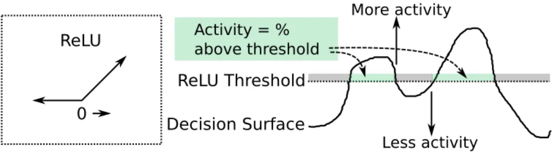
be achieved through the ReLU operations already present in many NNs. The NN’s output at any given layer may be made more or less sparse simply by moving the entire decision surface one direction or another through an auxiliary loss (Eq. (3.14)). . . 33

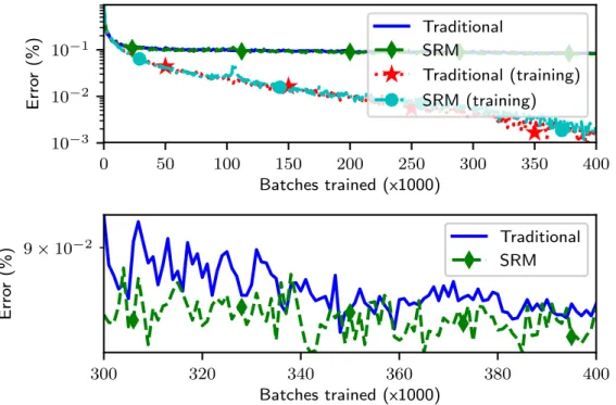
3.3 Example comparison on CIFAR-10 task between an SRM network

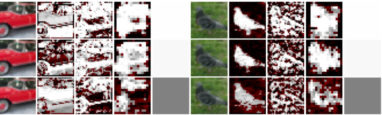
with a 90 % sparsity target and a traditional, non-SRM network. Each batch consisted of 64 training examples. . . 37 3.4 Example inputs (left), SRM activations before clipping (left-middle),

SRM activations after clipping (middle), and actual regions of input used for final classification (right-middle). The right-most image is the same visualization as the SRM outputs applied to a traditional NN that does not use point 3 of Section 3.2.2. . . 38 3.5 Saliency map given an input for both (a) original input, (b)

ran-dom perturbation, and (c) adversarial perturbation. Note that the saliency maps change drastically based on minor changes to the input. 40

3.6 Architecture of network, using GIM modules to produce an SRM. At top is the architecture for a traditional ResNet - note that the “GIM” modules do not exist in a traditional network, and are under-lined in red to note this. The inputs to an NN are typically already zero-mean and unit-variance, hence the lack of a batch normaliza-tion around the first GIM module. Within the Pre-block, the GIM is inserted between the two steps of the batch normalization opera-tion (normalizaopera-tion and the subsequent affine operaopera-tions, which are added to support a wider variety of output distributions). Within the GIM, a detached version of the information into the module is sent to a statistics network, which in turn produces a spatial mask by which features are multiplied, as per Section 3.3.2. The loss func-tion used to train the statistics network is specified in Secfunc-tion 3.3.2. 41

3.7 Example GIM activations on several images. The full-color images are the inputs; the following four columns are GIM activations be-fore the first, second, and third super blocks, and finally bebe-fore the global averaging layer. Only the third column of GIM activations were used to affect the network; the others were passive observers. Black indicates a GIM output of −1, red indicates a GIM output of just below zero, and white indicates a spatial location which was passed on to the final classification result, with a brighter white be-ing closer to 1. The three rows illustrate three different networks: one with λ = 0.9, another with λ = 0.99, and a third with both

λ = 0.99 and the learning rate for the GIM module set to 0.01 times the learning rate of the parent network, allowing for more gradual learning of relevance statistics. Note that the final column of each of these is a flat color, indicating no meaningful statistics were captured at that level. . . 46

4.1 While adversarial examples are considered a nuisance by most, they have the potential to provide reliable explanations with the same richness of information as the original input. For example, when an NN trained at finding lung nodules in radiographs needs investi-gation (a, b), an attack may be targeted at a desired new network output—such as changing a nodule classification to a non-nodule classification (c) or emphasizing the nodule (d)—to produce a new image which is minimally changed but produces the desired output. By comparing these inputs and looking at the differences, a human operator can identify relevant features in the input with greater fi-delity than current methods. . . 50 4.2 Compared to the state-of-the-art, our method achieved higher

ac-curacy while being tolerant of greater adversarial perturbations on both ImageNet (Fig. 4.2a) and CIFAR-10 (Fig. 4.2b). By measur-ing the ARA, a model’s resistance to adversarial attacks is taken into consideration alongside its ability to make predictions better than the naive baseline (the hatched region). See Section 4.1.1 for additional details. * Madry et al. used a network that was 10× as wide as a traditional ResNet-110, and also trained against an Linf

adversary rather than anL2 adversary [41]. †This curve came from

personal communication with A. Madry on a standard ResNet-50; see Section 4.1.1 for details. . . 54

4.3 A demonstration of LIME on an NN diagnosing lung nodules in the JSRT dataset. LIME’s algorithm consists of taking an input (a), dividing it up into super-pixels (b), and then using linear approxi-mations to determine which subset of super-pixels most significantly affects the network’s classification (c). How well does this explain the decision? . . . 58 4.4 Selvaraju et al.’s Grad-CAM [58] processes an input (a) and uses

back-propagation (b) to produce localized gradient information which can be presented as a heat map of salient regions (c). How well does this explain the decision? . . . 59 4.5 An adversarial example corresponding to the same network and

in-put as Figs. 4.3 and 4.4. Here, the resulting adversarial inin-put (a) is the sum of the original input (b) and a crafted noise term scaled by a small coefficient (c). The result is an imperceptible change in input leading to a completely different NN output. Also worth noting is that the location of the noise in (c) does not correlate well with either the LIME or Grad-CAM explanations. . . 60 4.6 In contrast to Fig. 4.5, our preliminary technique of increasing

ad-versarial distance concentrates the perturbations needed to change the network’s output. The RMSE (c) between the original input (a) and the adversarial attack (b) is also much greater for a smaller change in network output. . . 63 4.7 Example of emphasizing a lung nodule via the same method of

4.8 The previously mentioned attack ARA metric depends on the rel-ative confidence between the correct class and the second-most-confident class. For related classes such as “car” and “truck,” the distance between these two classes may not increase through train-ing. However, by measuring the distance from the correct class back to a fixed baseline, as is done with the BTR ARA metric, im-provements in feature recognition may be measured regardless of the presence of related classes. . . 67 4.9 Different explanation techniques using ρ = 0.075. (a) The

origi-nal image. (b) A positive explanation for the donut class; we note alignment of the added “hole” with a wrinkle in the original sand-wich bun. (c) A negative explanation for the donus class resulted in the removal of the round shape of the sandwich. (d) A positive explanation for the true class, sandwich, results in exposed contents (peppers or tomatoes), and the beginnings of lettuce. (e) A neg-ative explanation for the sandwich class reveals homogenization of the bun’s texture, and further rounding out of the overall shape. (f) Positive explanation for a completely unrelated class, horse; legs were clearly added, and the textured area in the upper-left of the image is appropriated as a saddle. . . 68

4.10 Training an NN on samples from a dataset (left) specify desired be-havior at the data points, but does not describe bebe-havior in between those data points, allowing the decision surface to take an arbitrary shape. Adding some noise (second from left) can somewhat improve the behavior between dataset samples, but is statistically unlikely to improve the worst behaviors. Adversarial training (second from right) deliberately attempts to improve the worst performing points, leading to a smoother decision surface. Adding a stochastic Lips-chitz loss, as Eq. (4.9), further smooths behavior between data points. 78 4.11 Prototype HITL interface. Whereas adversarial training simply

gen-erates adversarial examples and trains them to be recognized as the original class, our adversarial examples can be made of sufficient quality to merit human intervention as to whether or not the class of the image has changed. . . 80 4.12 Plot of all CIFAR-10 experiments run with a ResNet-44; accuracy on

clean data versus attack ARA (as per Section 4.2.1).

•

•

•

•

4.13 Input (left) and adversarial examples of different CIFAR-10 classes, generated for NNs with different levels of adversarial resistance using the different g(·) functions from Section 4.2.1, as indicated by the heading at the top of each column. The relative accuracy and attack RMSEs may be compared in Fig. 4.12; from top to bottom, these correspond to the experiments denoted by

•

•

•

•

4.14 TheL2,minmethod of adversarial generation adds stability to

adver-sarial training, but can suffer from degeneracy, where multiple train-ing examples of the same class override a lone neighbor of a different class. Here, L2,min adversarial training would result in “Class A”

being overshadowed by the two “Class B” instances. Since L2,min

stops at the border of a misclassification, the class with fewer lo-cal members only successfully trains a very narrow region. As per Paragraph 4.3.1.15.2, this may be fixed with HHAT. . . 101 4.15 A side-by-side comparison of the gexplain,+ explanations from a

net-work with the adversarial robustness modifications (top) versus with both adversarial robustness modification and the GIM SRM (bot-tom) shows that filtering out some of the intermediate activity of the network resulted in little change to the explanations. . . 108

4.16 Excerpt from the MEP-LINCS report delivered to OHSU. In the gray box are example images, unaltered, which were from the group treated with cxcl12|beta. Below that are three rows of images, each column being different views of the same image. Row 1 contains the adversarial example for cxcl12|beta using gexplain,+. Row 2 contains

the unaltered base image, and the ligand with which it was originally treated. Row 3 shows the difference between rows 1 and 2. . . 110

Glossary

Adversarial Attack / Adversarial Example:When a neural network is trained, it generates the correct output for some set of inputs. An adversarial attack is a modified version of an input for which the network would have been correct, but for the modified version, the network produces incorrect output. The perturba-tion from the clean input to the adversarial input is typically imperceptible for state-of-the-art networks. Since the perturbation is difficult for a human observer to detect, it may be used as an attack which makes the network fail in a way a human observer would not. More information may be found in Chapter 1.

AE: Adversarial Explanation. The most prominent contribution of this work, an adversarial explanation is an explanation which demonstrates features salient to the network’s classification in the same domain as the network input, and is produced via the same method as adversarial attacks. AEs are described in Chapter 4.

ARA: Accuracy-Robustness Area. On a graph with axes of allowable adversarial perturbation RMSE and classifier accuracy, the ARA is the area between a clas-sifier’s curve and the curve for a naive classifier. Since a non-naive classifier will always be susceptible to adversarial attacks of some magnitude, the ARA measures the decline in a classifier’s performance as progressively larger attacks are allowed. See Section 4.1.1 for additional information.

Attack ARA:ARA applied specifically to accuracy; that is, the “accuracy” axis used for the RMSE classification should be based on a top-1 classification accuracy.

See Section 4.1.1 for more information.

BTR: Better Than Random. For two classes which are closely related, the at-tack ARA is an unreliable measurement since the two classes are likely to gain confidence in tandem. BTR is therefore used to measure the difference between a class’ confidence and a random confidence value, as opposed to attack ARA, which measures the difference between the top two classes. See Section 4.2.1.2 for more information.

BTR ARA: The ARA metric computed with the accuracy axis replaced by the percentage of inputs where the correct class has greater than random confidence. See Section 4.2.1.2 for more information.

Explanation: In the context of this work, an explanation is a means of under-standing the decision made by an NN, ideally in a reliable way which requires minimal training to interpret. See Chapter 1 and Section 4.1.2 for comparisons amongst different state-of-the-art NN explanation methods.

GIM: Gradient Integration Module. A method for achieving a network bisection SRM by tracking gradient statistics in a secondary network. See Section 3.3.2 for more information.

HHReLU:Half-Huber Rectified Linear Unit. The methods outlined in Chapter 4 optimize the first derivative of the network’s output. A traditional ReLU function has a continuous value and a discontinuous first derivative, making optimization difficult. This may be eased by using a one-sided Huber function, which has both a continuous value and first derivative. See Section 4.2.4 for more information.

HITL:Human-In-The-Loop. Most supervised NNs are trained using inputs which have been annotated by human annotators. To improve the NN’s training, the data for more inputs must be gathered and these new inputs must then be labeled. HITL methods in this work refer to methods of improving a network’s training without requiring new data, instead leveraging communication between algorithms using the NN (such as AE) and a human observer. See Section 4.2.8 for more information.

LCA:Locally Competitive Algorithm. A sparse coding algorithm which minimizes the number of non-zero coefficients while simultaneously maximizing the fidelity of an input reconstruction based on the resulting sparse code. See Section 2.1 for more information.

ML: Machine Learning. Computer algorithms which learn without explicit pro-gramming. Rather than describing the input to output transformation explicitly, that transformation is learned based on examples of the desired function.

Network Bisection SRM: An SRM realized by bisecting an NN, and inserting an auxiliary loss at that point to enforce sparsity. Additional requirements and information is laid out in Chapter 3.

NN: Neural Network. An ML algorithm which combines layers of artificial “neu-rons,” which weight input signals, with non-linear activation functions. The result is a highly-parametrized model which can replicate a wide variety of functions.

ReLU:Rectified Linear Unit. An NN activation function which truncates negative values to zero, and leaves positive values unchanged.

RMSE: Root-Mean-Squared Error. A measurement of difference between two vectors, which is calculated by taking the square root of the mean of the squared difference between the elements in the vectors. Equal to the Euclidean distance between the two vectors normalized by the square root of the number of elements in the vectors.

SGD:Stochastic Gradient Descent. A method for training NNs which involves the repeated estimation of the network’s gradient with respect to some loss function, and then moving weights away from that gradient in an attempt to minimize the value of the loss function.

SRM: Sensory Relevance Model. A method of explaining an NN’s output which utilizes the same domain as the network’s inputs. By using the exact same format as the original input, a human observer may leverage their prior experience with the problem domain to analyze the NN’s decision in its original context, using changes between the explanation and the original input to infer relevance. This is in contrast to approaches which super-impose metadata on a sensory image, which may often be misinterpreted due to unclear relationships between the metadata and the original sensory domain. Two classes of SRM were explored: the network bisection SRM in Chapter 3, and adversarial explanations in Chapter 4.

1

Introduction

Deep learning is a fast-advancing technique for dealing with multidimensional in-put signals, including images and videos. The top performers for challenges such as ImageNet have been dominated by deep learning solutions [22], and the broad applicability of the technique has garnered usage across a swath of fields, including biomedical [24], logistics [40], user-recommendation engines [13], and defense [1]. Part of this popularity is owed to the genericism and simplistic efficiency of the approach: input signals are passed to highly-parallelizable computational layers that transform the data multiple times before producing output signals. The set of transformations possible in a sufficiently deep and wide network is infinite due to the repeated, non-linear activation functions. For this reason, deepNeural Net-works (NN) have been more effective on complicated problems than straightfor-ward Bayes’ approaches or other traditional Machine-Learning (ML) techniques. These output signals are in practice iteratively adjusted to minimize an arbitrary objective function via the popular backpropagation algorithm. This approach is extremely flexible: either the network’s output may be adjusted to approach some target signal, or the network’s output may optimize some task-specific heuristic.

To date, NN-based approaches have all been “black box” approaches, which im-pose no requirement for conveying intuition on the internals of the network. Many different internal architectures exist based on intuitive or beneficial properties, such as convolution or pooling layers, but the final interactions of these components are unrestricted and impossible to intuit. Furthermore, these networks tend to get

stuck in local minima that exist on the training set but not on test examples from the larger problem. This condition is known as over-fitting, and it can limit the ability of existing neural networks to achieve good performance on cases outside of the training set. An example of this phenomenon can be seen when training a net-work to classify a photo as containing an animal or not. Without efforts to prevent it, many instances of the network will learn to classify a blurry background as an animal, and a crisp background as not an animal, an artifact of the focal length for different types of photography [34]. For human operators, this “black box” quality makes debugging the systems - or improving them - a virtually impossible task.

Overall, the goal of this dissertation was to find a more reliable and informative way to explain the decisions made by neural networks. Here, “explain” means a method which demonstrates the reasoning behind a network’s output to a person, in such a manner that does not require the person to have expert training to interpret the explanation. A method of explanation should also have high fidelity to the model: that is, it should be unambiguous how the input would need to change to get a different result.

Current methods for debugging NNs are unreliable. The state-of-the-art for post-hoc network analysis involves investigating the internal layers via saliency maps [21, 59], or looking at the receptive fields to which internal nodes respond [4, 39, 47, 54, 58, 75]. Methods of modifying an NN’s architecture such that an “attention map” is both generated and used to filter inputs have also been pro-posed [12, 25, 28, 64]. In addition to generating compelling explanations, attention methods have been shown to improve network accuracy. However, as this disser-tation establishes, all of these existing methods share the same two flaws when considering their value for explaining network behavior.

Figure 1.1: Reproduction of Figure 3 from [28]. They proposed a very compelling, multi-level attention scheme which highlights salient objects wonderfully on the CIFAR-10 dataset. Fur-thermore, their scheme shows how the network’s attention is distributed at multiple levels within the network. Nonetheless, these highlights beg the question: within the regions marked salient, what qualities actually affect the network’s output?

The first flaw is demonstrated in this dissertation via adversarial attacks (also known as adversarial examples). Adversarial attacks are extremely small perturba-tions which completely change the network’s output; they are termed an “attack” because they may be used maliciously, for instance to make a turtle appear as a rifle [2]. Adversarial attacks against networks compatible with existing explana-tion methods have little to no correlaexplana-tion with the explanaexplana-tions generated by those methods. If an explanation were reliable, then the perturbations which change the network’s output should be related to that explanation. This is not the case for existing methods, drawing into question the importance of the regions highlighted by these explanation methods (Section 4.1.2).

The second flaw concerns the limited merit of heatmaps. Attention methods, such as Jetley et al.’s [28], produce extremely compelling masks of salient objects in the input (Fig. 1.1). However, while these do arguably show the region which most affected the network’s output (ignoring the first flaw of adversarial examples for the moment), they do not address the qualities of those regions that affect the output. In the third row of Fig. 1.1, for instance, who is to say that the network’s output was “deer” and not “dog?” Both classes would have roughly the same salient outline. From a human point of view, it would be easy to justify the explanation algorithm as including the antlers, but the algorithm itself highlighted a large region, the antlers being only a small portion of the overall explanation. Thus, the extent of the explanation’s benefit is to show that the salient object was considered, nothing about how or why it was considered. Existing explanation methods all focus on the generation of a heatmap, and all heatmap-based methods share this flaw (Section 3.4).

This dissertation proposesSensory Relevance Models(SRMs) as a means of ad-dressing the previously mentioned flaws, while also bringing deep learning closer to a form that can be reliably understood and manipulated by human operators. SRM refers to methods of explanation which utilize the same domain as the network’s sensory inputs. By using the exact same format as the original input, a human observer may leverage their prior experience with the problem domain to analyze the NN’s decision in its original context, using changes between the explanation and the original input to infer relevance.

For the first formulation of SRMs, network bisection, only the first of the above flaws were known. Adversarial examples affected any known method of explaining

an NN’s decision, even attention networks. From the very existence of impercep-tible adversarial examples, it may be inferred that NNs rely on very high gain factors from the input. Existing explanation methods were either post-hoc or attention-based, which multiplied all inputs by a small, but non-zero, coefficient. Attention-based examples were deemed a promising direction, and it was reasoned that filtering out spatial elements at different levels absolutely - multiplying by zero - would eliminate some of the input elements needed for adversarial attacks and focus the remaining attack into coherent features.

Counter-intuitively, explorations of the original SRM proposal resulted in ad-versarial examples with equivalent or even smaller perturbations. While investi-gating their spatial statistics yielded interesting salient regions at different levels in the network (Section 3.3.2), they utterly failed at the original goal of producing a reliable explanation mechanism. It seemed necessary to solve the mystery of why adversarial examples were not improved by this first iteration of SRMs, which utilized fewer input elements. Merely by the zeroing of some portion of inputs (up to 74 % on CIFAR-10), one might expect that the result would be adversarial examples of a larger magnitude. This was not the case. While investigating this phenomena, I also came to realize the second of the above flaws: heatmap-based methods do not possess the necessary richness to explain failure cases.

The failure of that first SRM led to a much more informative success: ad-versarial explanations (Chapter 4). The realization of the second flaw with ex-isting explanation methods necessitated a new method which would not rely on a heatmap. The original flaw necessitated an approach that worked alongside adversarial examples, or resulted in adversarial examples that aligned with the ex-planation. Consider the nature of a minimum-perturbation adversarial example:

Figure 1.2: State-of-the-art methods of explaining an NN’s decision based on some input (a) rely on the generation of some heatmap (b), generated here via Grad-CAM [58]. In cases where the object’s shape is non-discriminatory, this provides little insight into the decision. Adversarial examples produce much richer output, and can be leveraged to accentuate the NN’s decision (c), making salient features clearly visible when compared with the original image. Alternatively, some desired output may be encouraged to demonstrate features salient to that desired output (d). This technique also demonstrates training deficiencies - clearly, the COCO dataset contains few images of burgers from a top-down perspective, and a pile of ingredients is a strong indicator of sandwich-ness. Unless otherwise specified, all images in this paper were taken by the authors to avoid copyright issues.

it demonstrates the nearest decision boundary. That is, if adversarial examples themselves could consist of more significant perturbations, they would function as

definitive explanations. Adversarial examples have the capacity to illustrate the closest boundary, similarly to how other machine learning methods, such as trees, can be inspected for the closest boundary. To the best of my knowledge, this has not been proposed nor realized previously. The resulting work proposes a variety of techniques for enhancing the adversarial robustness of an NN. The work also demonstrates the efficacy of these techniques, not only surpassing the previous state-of-the-art defense against adversarial attacks by 2.4×, but also producing rich, full-color explanations that clearly illustrate the features considered salient by the network. The principle is demonstrated in Fig. 1.2. Compared to a state-of-the-art heatmap method, Grad-CAM [58], the adversarial explanations much more clearly demonstrate salient features and the reasoning behind the decision, and rely less on the human observer’s intuition to fill in missing information. This work was packaged into the attached paper, Appendix A.1.

Two new SRM techniques were proposed and analyzed in this dissertation. Network bisection is a novel form of attention which completely obscures parts of the input and is learned through an auxiliary loss, not directly through the classification loss. Adversarial Explanations (AE) are a novel group of techniques for stabilizing an NN such that adversarial attacks against that network are larger in magnitude and consist of coherent features.

The network bisection SRM formulation offered no benefits over other state-of-the-art work in its family. Newer techniques, such as the aforementioned Li

et al.[35] or Jetleyet al.[28] works on attention, have more pronounced benefits in terms of accuracy and HITL interaction when compared to the network bisection SRM. This dissertation also attempted a combination of the network bisection SRM formulation and the AE work. The results of the AE work were not enhanced

by the old SRM formulation, and were superior in every quantifiable and qualitative capacity.

The new AE techniques for robust networks and reliable explanations are un-paralleled at this time. They accomplish the same goals as the originally proposed SRM: increased adversarial resistance and a capacity for HITL interactions, as detailed in Chapter 4. Furthermore, they surpass the original expectations of this dissertation, as a fundamentally new way of investigating the operation of NNs. In contrast with previously proposed heatmap-based methods, including the net-work bisection SRM, the AE techniques provide higher-definition and more reliable feedback. As an added bonus, they demonstrate that classification networks may be used for generation, a machine learning niche previously occupied predomi-nantly byGenerative Adversarial Networks(GANs) and Variational Autoencoders

(VAEs).

1.1 Contributions

This work contains evidence of my work since the completion of my master’s degree in February 2016 [70], including:

1.1.1 Primary Contributions

• Proposed network bisection SRMs, a form of saliency maps that are inte-grated into the network (Chapter 3).

• Implemented network bisection SRMs via activity adjustment (Section 3.3.1) and gradient integration modules (Section 3.3.2). Demonstrated that SRMs can produce effective saliency maps which reveal key regions of the input

and work in a hierarchy, but that these shed little light on the final decision (Section 3.3).

• Established that network bisection SRMs do not increase resistance to ad-versarial attacks, due to increased variance in remaining pixels (Section 3.4).

• Created NN modifications and training strategies aimed at producing high-quality adversarial explanations, which improve on the state-of-the-art re-sistance to adversarial examples by 2.4×, and conducted a comprehensive ablation study of each modification (Chapter 4, [72], under peer review with Nature Machine Learning as in Appendix A.1).

• Improved adversarial training without other improvements by 17 %, in terms of both ability to resist adversarial attacks and produce explanations, via the

L2,min adversary (Paragraph 4.3.1.15.2 and Appendix A.1, [72]).

• Showed that adversarial examples could be used to produce reliable expla-nations with salient features (Chapter 4, [72]).

• Introduced theBetter Than Random(BTR)Accuracy-Robustness Area(ARA) quantitative metric, which correlated well with the quality of explanations produced (Section 4.2.1.2, [72]).

• Utilized adversarial examples as part of a Human-in-the-Loop workflow for enhancing network robustness against adversarial attacks (Chapter 4, [72]).

• Produced a report forOregon Health & Science University (OHSU)’s MEP-LINCS data on the effects of different ligand treatments on cell cultures in-vitro, based on the adversarial explanation methodology (Section 4.5).

1.1.2 Auxiliary Contributions

• Extended my M.S. thesis work, the Simple Spiking Locally Competitive Al-gorithm (SSLCA) [70], to include inhibition and an analysis of its efficacy when combined with modern deep learning techniques (Chapter 2; included as Appendix A.2, [69]).

• Proposed and evaluated four different architectures for performing vector matrix multiplication, a vital function for NNs, using memristors [68].

• Extended the training method for Rozell et al.’s Locally Competitive Algo-rithm(LCA) to combine supervised and unsupervised information, giving it better task-oriented effectiveness while still focusing on preserving the infor-mation contained in its inputs (Section 2.3).

• Partnered with UCLA to identify spoken digits, using an AgI atomic switch network as a computational reservoir (submitted). They made and tested the device, I formulated the experiments and analyzed the resulting data for computational ability.

• Applied the LCA to radiation detection as part of the Defense Threat Re-duction Agency (DTRA) program.

• Implemented a state-of-the-art deep learning classification pipeline, applied to many different problems include CIFAR-10, the Stanford Tower dataset, and OpenAI’s Gym’s CarRacing environment.

• Published 8 peer-reviewed papers, including:

– W. Woods and C. Teuscher, “Fast and Accurate Sparse Coding of Visual Stimuli with a Simple, Ultra-Low-Energy Spiking Architecture,” IEEE

Transactions on Neural Networks and Learning Systems, pp. 1-15, 2018 [69] (Appendix A.2).

– W. Woods et al., “Approximate Vector Matrix Multiplication Imple-mentations for Neuromorphic Applications using Memristive Crossbars,” IEEE NANOARCH, 2017 [68] (winner of the conference’s Best Paper award).

– K. Scharnhorst et al., “Non-Temporal Logic Performance of an Atomic Switch Network,” IEEE NANOARCH, 2017 [57].

– M. Tahaet al., “Approximate in-memory Hamming distance calculation with a memristive associative memory,” IEEE NANOARCH, 2016 [62].

– W. Woods, “The Design of a Simple, Spiking Sparse Coding Algorithm for Memristive Hardware,” Portland State University Master’s Thesis, 2016 [70].

– W. Woodset al., “Synaptic Weight States in a Locally Competitive Al-gorithm for Neuromorphic Memristive Hardware,” IEEE Transactions on Nanotechnology, 2015 [71].

– W. Woodset al., “Memristor panic - A survey of different device models in crossbar architectures,” IEEE NANOARCH, 2015 [73].

– W. Woods et al., “On the Influence of Synaptic Weight States in a Lo-cally Competitive Algorithm for Memristive Hardware,” IEEE NANOARCH, 2014 (winner of the conference’s Best Student Paper award) [67].

• Published 6 non-peer-reviewed proceedings, including:

Adversarial Examples on Robust Networks,” Portland State University Student Research Symposium, 2019.

– U. Khan, W. Woods, and C. Teuscher, “Exploring and Expanding the One-Pixel Attack,” Undergraduate Research & Mentoring Program, no. 34, 2019.

– J. H. Chen, W. Woods, and C. Teuscher, “Explanation Methods for Neural Networks,” Portland State University Student Research Sympo-sium, 2019.

– W. Woods, J. H. Chen, and C. Teuscher, “Explaining the Conclusions of Neural Networks,” Early Detection Conference at Oregon Health and Sciences University, 2018.

– J. H. Chen and W. Woods, “Generating Adversarial Attacks for Sparse Neural Networks,” Undergraduate Research & Mentoring Program, no. 31, 2018.

– J. Meng, C. Teuscher, and W. Woods, “Radiation Source Localization by using Backpropagation Neural Network,” Portland State University Student Research Symposium, 2018.

2

Locally Competitive Algorithm

The foundation of the SRM began via extensions to Rozell et al.’s LCA [55]. Sparsity was seen as an important factor for a useful explanation, consistent with insight into human explanations [45]. As a concept, the SRM never relied on the LCA, but the intrinsic sparsity properties of the LCA lent it as an excellent starting point for discussing the bisection of networks to produce intermediate output with semantic significance.

2.1 LCA

Our work on Rozell et al.’s LCA has led to a deep understanding of sparsity in ML [68, 69, 71]. Briefly, the LCA is a solution to the sparse coding problem: given anM ×N dictionary Φ consisting of N examples of an input space of dimension

M, how might an arbitrary inputs(t) be best represented as a linear combination of the columns of Φ? That is, an estimate of the input, ˆs(t), can be built via some coefficients a(t) as ˆs(t) = Φa(t). Solving the sparse coding problem involves devising some algorithmq(·) that mapsa(t) = q(s(t)). The sparse coding problem encapsulates the trade-offs between minimizing the number of non-zero coefficients in a(t) and the fidelity of ˆs(t) compared to the actual input s(t). Formally, the sparse coding problem may be posed as minimizing the following energy equation:

E(t) = 1

2||s(t)−sˆ(t)||

2 ₊X

m

whereλC(·) is a penalty term that, when large, emphasizes a small number of ac-tive coefficients, and when small, emphasizes fidelity in the reconstruction. Equa-tion (2.1) is minimized by the LCA [55].

The minimized energy equation, Eq. (2.1), demonstrates that sparse coding has a tuning knob,λ, which can be used to trade between higher coefficient sparsity or greater fidelity to the input. It has been theorized that sparse coding is an integral part of biological computation processes, due largely to the evidence of sparse coding activity in the mammalian cortex [42, 76]. As a result, many hardware implementations of the LCA have sprung up [7, 29, 30, 48, 50, 52, 53], including my own [69].

2.2 LCA and Deep Learning

Part of my attached paper on an LCA hardware implementation (Appendix A.2, [69]) involved comparing the accuracy of deep learning models trained both on raw data and on LCA-encoded data. Despite biological backing for sparsity, the LCA always reduced the accuracy of the deep learning model. While the LCA solves the sparse coding problem, it relies on a dictionary that is trained on example inputs using unsupervised training. This unsupervised training typically derives from Oja’s rule [46], which updates elements participating in the reconstruction such that subsequent reconstructions will be more accurate:

Φt+1 = Φt+µ(s(t)−sˆ(t))aT. (2.2)

dictionary trained via this method, potentially discarding information which would be helpful for classification in favor of information which decreases theL2 distance

between the original input and the reconstruction.

Regardless of lost accuracy, the potential benefits of the LCA became clear through this work. The LCA identifies prominent features in its input, and greatly reduces the non-zero dimensionality of its output. One issue with investigating NNs is that, in a typical convolutional layer, far too many elements in the convolution are non-zero to visualize what the network is considering. With an LCA, the number of non-zero elements is so low that they can be visualized. We discuss adapting the LCA as the base of the SRM, while simultaneously addressing the loss in accuracy, in Section 2.3.

2.3 Supervised LCA

The LCA traditionally uses unsupervised learning. As its operation is defined en-tirely through reconstructing its input, unsupervised learning is a natural fit. How-ever, unsupervised operation has its trade-offs. While unsupervised approaches tend to learn quickly, they never perform as well as task-specific (supervised) approaches. Rather than making all of their parameters available for the final objective, they are instead attempting to solve a completely different task: re-representing their input. On the other hand, supervised approaches attempt to transform their input for a single purpose, with each transformation bringing the data in the network closer to the desired output. Supervised learning is required to solve the overall information processing problem. This is where SRMs come in as a middle ground: we implemented a system that cleans up the input in a task-specific manner, while also preserving and compressing qualities of the input

to make the results more sensible to manipulate.

To consider using an LCA with backpropagation, we must be able to define the output of the network in terms of its inputs. This is due to the derivatives required for backpropagation to function. However, the LCA’s operation is traditionally defined in reverse, where the input may be reconstructed as a linear combination of dictionary elements. Manipulating this expression using the Gramian leads to:

s(t)≈Φ(t)a(t),

ΦT(t)Φ(t)−1ΦT(t)s(t)≈a(t). (2.3)

Taking the true derivative of Eq. (2.3) with respect to each weight inΦ(t) would be cumbersome and expensive due to the inverse, which may either be unstable or not exist if all dictionary elements are not sufficiently independent of each other. Instead, we replace the Gramian with its diagonal approximate, propagating the scalar derivative of each element in turn:

ΦT(t)Φ(t)−1 ΦT(t)s(t)≈a(t), ||Φi(t)||−22ΦTi (t)s(t)≈ai(t), −P j2Φj,i(t)∂Φj,i(t) ||Φi(t)||42 ΦT_i (t)s(t) +||Φi(t)||−22∂ΦTi (t)s(t)≈∂ai(t), (2.4)

To show the efficacy of this approach, we have compared the traditional, un-supervised method of training the LCA with this novel, un-supervised method of training an LCA. Each network compared consisted of a single LCA layer with a

0 20 40 60 80 100 120

Samples Trained (thousands)

0 20 40 60 80 Accuracy (%) _{Unsupervised LCA} Supervised LCA

Supervised + Unsupervised LCA

Figure 2.1: Supervised extension to the LCA vs its original, unsupervised formulation.

dictionary represented by 50 neurons followed by a single perceptron layer with 10 neurons for classification on the MNIST digit database. Results are shown in Fig. 2.1. Note that the traditional, unsupervised approach quickly reaches its maximum performance, and then hovers at that level or even loses some ability to classify the input due to its emphasis on reconstructing the input well rather than classifying the input well.

On its own, the supervised gradient is incapable of training the LCA. A purely supervised approach breaks down due to the conflict between the supervised loss we derived above and the sparse coding equation intrinsically minimized by the LCA (Eq. (2.1)). The incompatibility of these two terms causes the columns of Φ to become degenerate, leading to a collapse of the network’s functionality. However, combining the supervised gradient with the unsupervised gradient results in a more stable and higher-accuracy network configuration. This indicates that the LCA, which reconstructs an input stimulus based on a limited number of prominent features, can be adjusted to reconstruct the input stimulus based on task-specific

features. The two loss functions together eliminate the reduced accuracy of using a sparse coding layer while retaining its sparsity properties.

2.4 Extending the Supervised LCA to SRMs via Network Bisection

The supervised version of the LCA was functionally a bisected network with two parts: one responsible for generating a task-oriented sparse code of the input, and another for converting the resulting code into a decision regarding the input. This was the underlying theory of SRMs as originally proposed: suppress irrelevant aspects of the input, forwarding only those that would affect the prescribed task. Furthermore, since we derived a task-oriented gradient, we could use that gradient to manipulate the LCA independently of the overall network. This was the key implementation idea behind manipulating the SRM: it is feasible to descend both the loss function for the overall task as well as an auxiliary loss function applied only to the intermediate output from the network, which might be defined by a human operator. In this way, the sparse output of the SRM, which might be implemented via an LCA on top of other processing layers, could both be used to investigate the operation of the network at an intermediate step and to guide its processing.

The first proposed method for achieving an SRM therefore involved a poten-tially iterative procedure for bisecting the network into two pieces: one which generated a sparse, intermediate representation, and the second which generated a classification based off of that intermediate representation. While the first for-mulation for realizing SRMs had many similarities to attention-based neural net-works [12,28,64], it was unique for two reasons: first, the mask was learned through backpropagation via an auxiliary loss separate from the classification loss; second,

the mask generated by the proposed SRM would exist in a transformed feature space congruent with the input space but potentially scaled or richer in features. This would allow for a much sparser output than typically seen with attention-based neural networks. In the context of adversarial examples, zeroing much of the input would render high gain on those masked regions irrelevant. Elegantly, this approach was motivated by the knowledge that mammalian brains explicitly process saliency as part of processing visual scenes [27]. It was also proposed that the intermediate region could be “painted” by a human operator, a form of

Human-in-the-Loop (HITL) learning. This HITL aspect was validated by recent, promising work with redirecting the salient region in an attention model based on segmentation annotations [35]. That work, by Li et al., was made public on Feb. 27th, 2018, four days after the original proposal for this dissertation.

Our prior work with LCAs also points to a larger and more significant general problem: how sparse can the input to a classifier be to still achieve a given level of performance? This question is addressed in Section 3.4, though the answer depends heavily on the problem being solved. To intuit the relation between sparsity and ease of explanation, consider the problem of dictionary definitions. While many definitions could be substantially longer to capture more connotations and usages, and thus be slightly more accurate, a shorter definition is easier to understand. Similarly, I wanted to generalize this idea to all two-stage information processing pipelines. I observe that constricting the information shared between these two pipelines to be as sparse as possible, while also preserving locality of the sparse output, will generate a relevance mapping where the few non-zero elements indicate significant information for the task implemented by the pipeline. Functionally, this is similar to an autoencoder, but differs in a few ways: the dimension of the

middle layer does not need to be smaller to be constricting, as we use a sparsity loss to achieve a similar effect, and the second half of the network is not trying to reconstruct the input, but is rather trying to accomplish a different task.

3

Sensory Relevance Models via Network Bisection(s)

The general task of information or signal processing can be modeled as a function that converts some input space X to some different output spaceY. This input-output mapping is loosely defined on purpose for most methods so that they may have a broad applicability. For NNs, this generality has come at the cost of being unable to intuit how the mapping function works.

Adequately understanding the internal operation of NNs, or the larger toolbox of ML solutions in general, has recently become a primary difficulty of using them [14]. Complications arising from the internal flexibility of NNs are epitomized in adversarial examples: inputs with minor perturbations that completely change the output of the network [2,10,15,61,63]. These reports all support that NNs solve an underconstrained problem: many possible solutions to the training data exist on manifolds which are distorted toward imperceptibility in standard visual space. As such, overall accuracy on a sample dataset of an overall problem has become less important than an ability to reason about the scope and function of ML techniques. There have been both procedural and architectural attempts at understanding the behavior of NNs as well as making them more resistant to adversarial examples; Section 3.1 details these.

I add SRMs via Network Bisection to the field of explanation techniques. In this case, the X → Y transformation is split up into a two-stage process, such that an intermediate result is created, the SRM denoted as S(X). Since the network’s transformation is now defined as S(X) → Y, an intuitive and reliable

method of visualizing the SRM output would allow for unambiguous confirmation of the aspects being considered by the NN. This work sought to answer: if all information transmitted to the classifier were visualizable in a robust manner, would that visualization be useful for debugging the network? Network bisection is detailed throughout the rest of this chapter.

3.1 Related Work

Procedural attempts at understanding NNs primarily fall under the category of either saliency maps or investigating receptive fields. Saliency maps are produced by running back-propagation all the way to the input layer, and looking at which pixels are most influential on the network’s output [59]. This approach has proven useful for demonstrating what parts of the input are most important to a neural network. Saliency maps have also been extended to aid in image segmentation [21, 59]. By combining saliency maps from multiple, convolved classifications of a source image, saliency maps have even been used to track an object across time by updating the prior of the object’s position according to computed saliency maps [21]. Studies of receptive fields have been primarily limited to investigating the input patterns to which neurons at different levels in an NN respond [39,47,75]. By looking at these patterns, researchers have hoped to gain an intuition of the internal functions of the networks.

However, as will be demonstrated further in Chapter 4, these post-hoc meth-ods of explaining an NN’s intuitions suffer from incompatibility with adversarial examples, perturbations of a small enough magnitude that they are invisible to a human observer. The adversarial modifications do not correlate with the previ-ously mentioned methods of explanation, and as such calls such explanations into

question.

Training modifications to make NNs more robust to adversarial inputs have been proposed. A. Madry et al.have published several works on adversarial train-ing, integrating adversarial examples into the training process to make a network more robust [41, 63]. Columbia University’s DeepXplore project is another project that utilizes adversarial training; in their work, Pei et al. consider the automatic generation of adversarial examples, and using these generated examples to increase the training pool of the network [51]. Doing so forces the network to become a better generalizer as adversarial examples are actively trained away. However, this approach takes a significant amount of time, and while it is guaranteed to improve a network’s resistance to adversarial examples, it remains very difficult to prove an absence of adversarial examples. Likely, the neighborhood of possible adversarial attacks exceeds the bounds tested by DeepXplore. One might imagine adversarial attacks defined specifically closer to the boundaries of the network’s decisions than a project like DeepXplore generates. Realistically, there are limits on how much training a DeepXplore-like system can utilize, due to time and resource constraints. A prior architectural extension of network design to make NNs more under-standable is attention models [12, 64]. Where saliency maps demonstrate the most-used pixels, attention models use a gating technique which involves mul-tiplying the inputs by a learned mask to shape how inputs are forwarded to the classifying portion of the network. Viewing the mask of the attention model shows which inputs were weighted more heavily for a given input. My proposed network bisection differs from attention models because network bisection transforms the input while keeping it local, a much richer approach than the input gating ap-proach used by traditional attention models (attention models from the last year

have also incorporated this quality, e.g. [28]). Additionally, the network bisection technique uses a method separate from classification loss to enforce sparsity in the attentive layer (Section 3.3).

Outside of attempts to understand NNs and harden them against adversarial examples, there are two developmentally significant seeds for the network bisection SRM: one is the our work on Rozellet al.’s LCA [55], and the other is GANs [14]. The LCA was covered in Chapter 2.

GANs, introduced by Goodfellow et al. in 2014, rely on competition between two NNs attempting to optimize different loss functions: a generator, which gen-erates outputs similar to some reference input, and a discriminator, which takes inputs from the generator and real inputs and attempts to discern which input was real and which was generated [14]. As the discriminator learns to better recognize real inputs, the generator must improve at generating fakes of the input. As the generator learns to create better fake inputs, the discriminator must improve at telling the two apart. Together, these networks compute a loss function that would be impossible to design holistically. The network bisection SRM can be thought of similarly: one network, the SRM, has the goal of transforming its input into a maximally sparse output, while the second network, a classifier, must perform classification based on the limited information passed by the SRM. While comput-ing an optimal SRM directly would be impossible, computcomput-ing it in tandem with a corresponding output classifier makes the problem we are trying to solve feasible.

3.2 Theory

I proposed network bisection as a means of applying more structure to theX →Y transformation, such that an intermediate result, the SRM denoted asS(X), would

SRM Innovations

Easier to modify

Easier to interpret

Closer to how we learn Input Ultrasound Traditional Target Mask

SRM

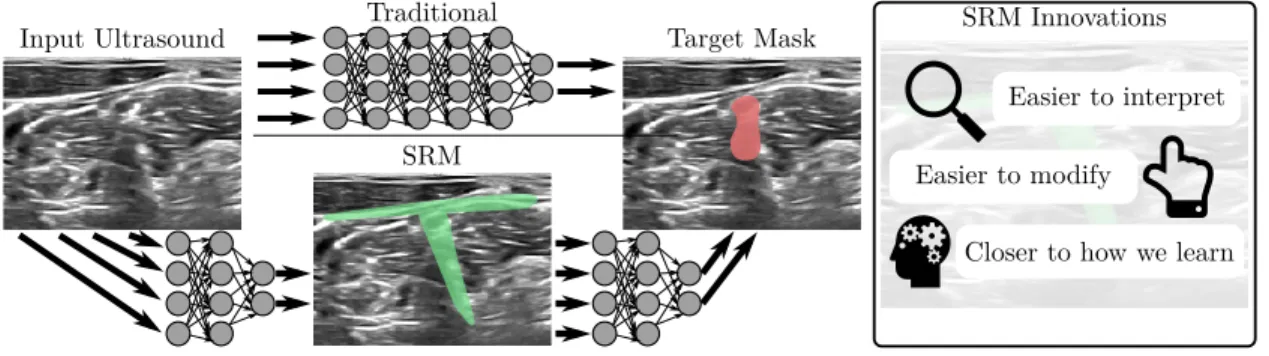
Figure 3.1: SRMs via network bisection sought to provide an intermediate, compressed represen-tation of input signals that would be useful for human-in-the-loop debugging of data processing algorithms.

provide better insight into the mechanisms of the overall transformation. The reasoning for bisection, and the necessary qualities of that bisection, are detailed in this section.

3.2.1 Why Bisection?

The proposed architecture is illustrated in Fig. 3.1. Similar to the GANs devel-oped by Goodfellow et al. [14], the SRM combines two separate machine learning methods solving different, but related, problems. GANs are implemented in terms of a generator, which transforms noise into a believable image, and a discriminator, which takes one real image and one from the generator, and attempts to discern which is the real image. A problem utilizing a network bisection SRM, on the other hand, is implemented in terms of the SRM, which attempts to forward as little information as possible, and a classifier, which attempts to score highly on a given task based only on the input from the SRM. The composition of these two networks solves the original information processing task.

Bisection SRMs necessarily can only express a subset of the operations available with current state-of-the-art deep NNs. The SRM technique requires restricting

some of the free dimensions of the NN; given enough input data (to prevent over-fitting and ensure generalization), an unrestricted network would almost certainly outperform the SRM formulation. On the other hand, convolutional layers are also less expressive than fully-connected NNs, yet they have led to significantly more accurate and robust networks [32].

Unrestricted networks are also known to be highly vulnerable to adversarial attacks. Consider the recent work on ArXiv from MIT’s LabSix group [2]. This group managed to 3D-print objects that Google’s Inception network would mis-classify. For example, they 3D-printed a turtle model that always registered as a rifle when passed to Google’s classifier, regardless of orientation [2]. This is a significant problem: traditional neural networks cannot be used in production for critical applications with such glaring flaws.

Restricting the input space of NNs has shown some promise at reducing the effectiveness of adversarial attacks [19]. This was the SRM’s first potential benefit over a traditional NN. The traditional NN might be learn to be more accurate with enough data but should also be significantly easier to manipulate. By restricting the intermediate space through sparsity, a bisection SRM would eliminate several vectors of reasoning that would prevent it from generalizing well. In contrast to attention models, where NNs may still utilize high gain on elements which are scaled as unimportant, the bisection SRM would completely mask out elements, giving them zero influence on the final network decision.

The second proposed unique benefit of the SRM arose from its construction as two separate pieces. Consider how people learn to solve problems and generalize well. Studies on student learning have investigated the differences between how experts and novices approach problems [60]. These studies tend to conclude that

experts develop a repertoire of “schemas” which can be applied to filter larger problems into a manageable (and efficient to solve) set of smaller problems [60]. The overall result, in the context of humans, is that a novice with the proper tools can solve the same problems as an expert, but far less efficiently and with greater cognitive stress [60]. A more recent study compares learning between students given feedback in the form of worked examples or tutoring versus basic correctness feedback [43]. Similarly, McLaren et al. conclude that providing worked examples as opposed to only correctness feedback greatly improved the efficiency of learning, but not the overall accuracy of the material learned [43].

Applied to information processing tasks, this implies that an efficient means of teaching generalizable solutions might require access to worked solutions. While part of what makes NNs so widely applicable is their genericism, and the fact that designing a system only requires constructing input-output pairs and a network architecture, this is also likely what is holding back further understanding and development of the function space realizable by NNs. By formulating the SRM as a local, sparse transformation of the input, it is guaranteed that the output could be interpreted by a human operator. This was the fundamental requirement of our system: that a human expert be able to see, given some input, which parts of that input were used to make the final classification. As this middle layer would be visualizable, tools could be developed to manipulate the SRM layer directly, changing the system’s idea of which parts of a given input are relevant, and adjusting the classification layer accordingly to rely on only the input information that is most significant.

this could have enabled a new type of feedback unexplored by previous NN ar-chitectures. Prior efforts to counter-act adversarial examples have been limited to generating adversarial examples and training the network to classify them cor-rectly [41, 51], or restricting the input space dicor-rectly, without concern to how this might affect the overall task [19]. Bisection SRMs would allow a human operator to directly point out which part of the input space is the most important, signif-icantly reducing the possibility of the network honing in on the wrong aspect of the input, and improving its ability to generalize.

3.2.2 Required Traits

The implementation of the bisection SRM relied on defining two sub-problems of the greater information processing problem. A formal definition of the overall task of our system relied on some desired functionY =f(X), where Y is theM -dimensional output space of the problem, andX is theN-dimensional input space. Our task is to find an approximate ˆY = ˆf(X) that minimizes some lossL[Y,Yˆ]. The SRM arose by defining ˆf(X) = C(S(X)), where C is the final classifier that shapes the output of the SRM, S. We then could define loss functions for each of these:

L_S[S(X)] =gλC(S(X)), L[Y,Yˆ],

L_C[C(S(X))] =L[Y,Yˆ], (3.1)

where λC(·) has the same meaning as in Eq. (2.1) of the LCA, a sparsity penalty term, and g(·) is a function to combine the sparsity and classifier output losses (often a weighted sum). Note that, if a desired SRM output ˆS(x) is specified, and

L[S(X),Sˆ(X)] is defined as the Mean-Square-Error (MSE) between the norms per unit-space of X of the two, then both stages of the pipeline may have their respective losses minimized. This would enable a human operator to specify an ideal SRM output and simultaneously converge the SRM to recognize that region as relevant and convergeC to perform the desired task using only that information. This exact approach was shown to be practical by Li et al., who used the Grad-CAM algorithm as a basis rather than network bisection [35].

Ignoring the other requirements of an SRM for a moment, we earlier demon-strated a combined loss function on S(X) of g(a, b) = a+b in Fig. 2.1. Indeed, what was derived in that work could be considered a proto-SRM. However, that model possessed neither the locality nor the correct form of sparsity required for a true SRM. To address this gap, we apply three restrictions toS(X):

1. The output must be in a similar space to X.

2. Each element of the output must rely primarily on inputs local to its spatial point.

3. Sparsity of the output alone is an insufficient restriction; sparsity must be evaluated in the original space ofX.

Point 1 refers to the similarity between the output space ofX andS(X). One of the primary purposes of the network bisection SRM was to make it easier to interpret what an ML technique is deeming relevant. In this light, the SRM could be thought of as a saliency map with an extra dimension containing transformed values that are fed into the final classifier. As such, the ability to re-cast the output to the original space to render overlays is imperative. An important note, if the input is a 32×32×3Red-Green-Blue(