Sparse Overcomplete Word Vector Representations

Sparse Overcomplete Word Vector Representations

Manaal Faruqui Yulia Tsvetkov Dani Yogatama Chris Dyer Noah A. Smith Language Technologies Institute

Carnegie Mellon University Pittsburgh, PA, 15213, USA

{mfaruqui,ytsvetko,dyogatama,cdyer,nasmith}@cs.cmu.edu

Abstract

Current distributed representations of words show little resemblance to theo-ries of lexical semantics. The former are dense and uninterpretable, the lat-ter largely based on familiar, discrete classes (e.g., supersenses) and relations (e.g., synonymy and hypernymy). We pro-pose methods that transform word vec-tors into sparse (and optionally binary) vectors. The resulting representations are more similar to the interpretable features typically used in NLP, though they are dis-covered automatically from raw corpora. Because the vectors are highly sparse, they are computationally easy to work with. Most importantly, we find that they out-perform the original vectors on benchmark tasks.

1 Introduction

Distributed representations of words have been shown to benefit NLP tasks like parsing (Lazari-dou et al., 2013; Bansal et al., 2014), named en-tity recognition (Guo et al., 2014), and sentiment analysis (Socher et al., 2013). The attraction of word vectors is that they can be derived directly from raw, unannotated corpora. Intrinsic evalua-tions on various tasks are guiding methods toward discovery of a representation that captures many facts about lexical semantics (Turney, 2001; Tur-ney and Pantel, 2010).

Yet word vectors do not look anything like the representations described in most lexical seman-tic theories, which focus on identifying classes of words (Levin, 1993; Baker et al., 1998; Schuler, 2005) and relationships among word meanings (Miller, 1995). Though expensive to construct, conceptualizing word meanings symbolically is important for theoretical understanding and also

when we incorporate lexical semantics into com-putational models where interpretability is de-sired. On the surface, discrete theories seem in-commensurate with the distributed approach, a problem now receiving much attention in compu-tational linguistics (Lewis and Steedman, 2013; Kiela and Clark, 2013; Vecchi et al., 2013; Grefen-stette, 2013; Lewis and Steedman, 2014; Paperno et al., 2014).

Our contribution to this discussion is a new, principled sparse coding method that transforms any distributed representation of words into sparse vectors, which can then be transformed into binary vectors (§2). Unlike recent approaches of incorpo-rating semantics in distributional word vectors (Yu and Dredze, 2014; Xu et al., 2014; Faruqui et al., 2015), the method does not rely on any external information source. The transformation results in longer, sparser vectors, sometimes called an “over-complete” representation (Olshausen and Field, 1997). Sparse, overcomplete representations have been motivated in other domains as a way to in-crease separability and interpretability, with each instance (here, a word) having a small number of active dimensions (Olshausen and Field, 1997; Lewicki and Sejnowski, 2000), and to increase stability in the presence of noise (Donoho et al., 2006).

Our work builds on recent explorations of spar-sity as a useful form of inductive bias in NLP and machine learning more broadly (Kazama and Tsu-jii, 2003; Goodman, 2004; Friedman et al., 2008; Glorot et al., 2011; Yogatama and Smith, 2014,

inter alia). Introducing sparsity in word vector di-mensions has been shown to improve dimension interpretability (Murphy et al., 2012; Fyshe et al., 2014) and usability of word vectors as features in downstream tasks (Guo et al., 2014). The word vectors we produce are more than 90% sparse; we also consider binarizing transformations that bring them closer to the categories and relations of

ical semantic theories. Using a number of state-of-the-art word vectors as input, we find consis-tent benefits of our method on a suite of standard benchmark evaluation tasks (§3). We also evalu-ate our word vectors in a word intrusion experi-ment with humans (Chang et al., 2009) and find that our sparse vectors are more interpretable than the original vectors (§4).

We anticipate that sparse, binary vectors can play an important role as features in statistical NLP models, which still rely predominantly on discrete, sparse features whose interpretability en-ables error analysis and continued development. We have made an implementation of our method publicly available.1

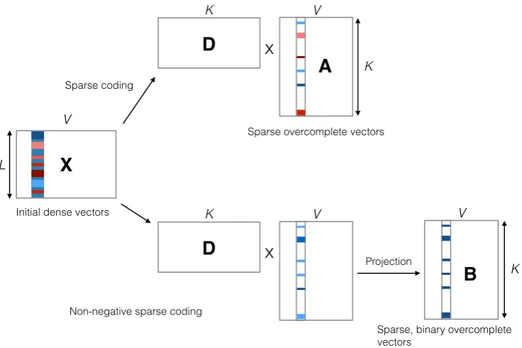
2 Sparse Overcomplete Word Vectors We consider methods for transforming dense word vectors to sparse, binary overcomplete word vec-tors. Fig. 1 shows two approaches. The one on the top, method A, converts dense vectors to sparse overcomplete vectors (§2.1). The one beneath, method B, converts dense vectors to sparse and bi-nary overcomplete vectors (§2.2 and§2.4).

LetV be the vocabulary size. In the following, X ∈ RL×V _{is the matrix constructed by} stack-ing V non-sparse “input” word vectors of length

L (produced by an arbitrary word vector estima-tor). We will refer to these as initializing vectors. A∈RK×V _{containsV sparse overcomplete word} vectors of lengthK. “Overcomplete” representa-tion learning implies thatK > L.

2.1 Sparse Coding

In sparse coding (Lee et al., 2006), the goal is to represent each input vector xi as a sparse linear combination of basis vectors,ai. Our experiments consider four initializing methods for these vec-tors, discussed in Appendix A. GivenX, we seek to solve

arg min

D,A kX−DAk

2

2+λΩ(A) +τkDk22, (1)

whereD ∈ RL×K _{is the dictionary of basis} vec-tors.λis a regularization hyperparameter, andΩis the regularizer. Here, we use the squared loss for the reconstruction error, but other loss functions could also be used (Lee et al., 2009). To obtain sparse word representations we will impose an`1

1_{https://github.com/mfaruqui/}

sparse-coding

penalty onA. Eq. 1 can be broken down into loss for each word vector which can be optimized sep-arately in parallel (§2.3):

arg min

D,A

V

X

i=1

kxi−Daik22+λkaik1+τkDk22 (2)

wheremidenotes theith column vector of matrix M. Note that this problem is not convex. We refer to this approach asmethod A.

2.2 Sparse Nonnegative Vectors

Nonnegativity in the feature space has often been shown to correspond to interpretability (Lee and Seung, 1999; Cichocki et al., 2009; Murphy et al., 2012; Fyshe et al., 2014; Fyshe et al., 2015). To obtain nonnegative sparse word vectors, we use a variation of the nonnegative sparse coding method (Hoyer, 2002). Nonnegative sparse coding further constrains the problem in Eq. 2 so thatDandai are nonnegative. Here, we apply this constraint only to the representation vectors{ai}. Thus, the new objective for nonnegative sparse vectors be-comes:

arg min

D∈RL×K

≥0 ,A∈RK≥0×V

V

X

i=1

kxi−Daik22+λkaik1+τkDk22

(3) This problem will play a role in our second ap-proach,method B, to which we will return shortly. This nonnegativity constraint can be easily incor-porated during optimization, as explained next. 2.3 Optimization

We use online adaptive gradient descent (Ada-Grad; Duchi et al., 2010) for solving the optimiza-tion problems in Eqs. 2–3 by updatingAandD. In order to speed up training we use asynchronous updates to the parameters of the model in parallel for every word vector (Duchi et al., 2012; Heigold et al., 2014).

However, directly applying stochastic subgradi-ent descsubgradi-ent to an `1-regularized objective fails to produce sparse solutions in bounded time, which has motivated several specialized algorithms that target such objectives. We use the AdaGrad vari-ant of one such learning algorithm, the regular-ized dual averaging algorithm (Xiao, 2009), which keeps track of the online average gradient at time

t:g¯t = 1_tPtt0₌₁gt0 Here, the subgradients do not

X

L

V

K

x

V

D

A

K

x

V

D

V

K

B

Sparse overcomplete vectors

Sparse, binary overcomplete vectors

Projection Sparse coding

Non-negative sparse coding Initial dense vectors

Figure 1: Methods for obtaining sparse overcomplete vectors (top, method A,§2.1) and sparse, binary overcomplete word vectors (bottom, method B,§2.2 and§2.4). Observed dense vectors of lengthL(left) are converted to sparse non-negative vectors (center) of lengthKwhich are then projected into the binary vector space (right), whereL K. Xis dense,Ais sparse, andBis the binary word vector matrix. Strength of colors signify the magnitude of values; negative is red, positive is blue, and zero is white.

with respect toai. We define

γ =−sign(¯gt,i,j)p_Gηt

t,i,j(|g¯t,i,j| −λ),

whereGt,i,j = Ptt0₌₁g2_t0_,i,j. Now, using the

av-erage gradient, the`1-regularized objective is op-timized as follows:

at+1,i,j =

(

0, if|g¯t,i,j| ≤λ

γ, otherwise (4)

where,at+1,i,j is thejth element of sparse vector ai at the tth update and g¯t,i,j is the correspond-ing average gradient. For obtaincorrespond-ing nonnegative sparse vectors we take projection of the updatedai ontoRK

≥0by choosing the closest point inRK≥0 ac-cording to Euclidean distance (which corresponds to zeroing out the negative elements):

at+1,i,j=

    

0, if|g¯t,i,j| ≤λ

0, ifγ <0

γ, otherwise

(5)

2.4 Binarizing Transformation

Our aim with method B is to obtain word rep-resentations that can emulate the binary-feature

X L λ τ K % Sparse

Glove 300 1.0 10−5 _{3000 91} SG 300 0.5 10−5 _{3000 92}

GC 50 1.0 10−5 _{500 98}

Multi 48 0.1 10−5 _{960 93} Table 1: Hyperparameters for learning sparse overcomplete vectors tuned on the WS-353 task. Tasks are explained in§B. The four initial vector representationsXare explained in§A.

hot, fresh, fish, 1/2, wine, salt series, tv, appearances, episodes 1975, 1976, 1968, 1970, 1977, 1969 dress, shirt, ivory, shirts, pants upscale, affluent, catering, clientele

Table 2: Highest frequency words in randomly picked word clusters of binary sparse overcom-plete Glove vectors.

state this as an optimization problem:

arg min

D∈RL×K B∈{0,1}K×V

V

X

i=1

kxi−Dbik22+λkbik11+τkDk22

(6) whereBdenotes the binary (and also sparse) rep-resentation. This is an mixed integer bilinear pro-gram, which is NP-hard (Al-Khayyal and Falk, 1983). Unfortunately, the number of variables in the problem is≈ KV which reaches100million when V = 100,000and K = 1,000, which is intractable to solve using standard techniques.

A more tractable relaxation to this hard prob-lem is to first constrain the continuous represen-tationAto be nonnegative (i.e, ai ∈ RK≥0;§2.2). Then, in order to avoid an expensive computation, we take the nonnegative word vectors obtained us-ing Eq. 3 and project nonzero values to1, preserv-ing the 0 values. Table 2 shows a random set of word clusters obtained by (i) applying our method to Glove initial vectors and (ii) applyingk-means clustering (k= 100). In§3 we will find that these vectors perform well quantitatively.

2.5 Hyperparameter Tuning

Methods A and B have three hyperparameters: the

`1-regularization penalty λ, the `2-regularization penaltyτ, and the length of the overcomplete word vector representationK. We perform a grid search onλ ∈ {0.1,0.5,1.0}andK ∈ {10L,20L}, se-lecting values that maximizes performance on one “development” word similarity task (WS-353, dis-cussed in§B) while achieving at least 90% sparsity in overcomplete vectors. τ was tuned on one col-lection of initializing vectors (Glove, discussed in

§A) so that the vectors in D are near unit norm. The four vector representations and their corre-sponding hyperparameters selected by this proce-dure are summarized in Table 1. There hyperpa-rameters were chosen for method A and retained for method B.

3 Experiments

Using methods A and B, we constructed sparse overcomplete vector representations A, starting from four initial vector representations X; these are explained in Appendix A. We used one bench-mark evaluation (WS-353) to tune hyperparame-ters, resulting in the settings shown in Table 1; seven other tasks were used to evaluate the quality of the sparse overcomplete representations. The

first of these is a word similarity task, where the score is correlation with human judgments, and the others are classification accuracies of an ` 2-regularized logistic regression model trained using the word vectors. These tasks are described in de-tail in Appendix B.

3.1 Effects of Transforming Vectors

First, we quantify the effects of our transforma-tions by comparing their output to the initial (X) vectors. Table 3 shows consistent improvements of sparsifying vectors (method A). The exceptions are on the SimLex task, where our sparse vectors are worse than the skip-gram initializer and on par with the multilingual initializer. Sparsification is beneficial across all of the text classification tasks, for all initial vector representations. On average across all vector types and all tasks, sparse over-complete vectors outperform their corresponding initializers by 4.2 points.2

Binarized vectors (from method B) are also usu-ally better than the initial vectors (also shown in Table 3), and tend to outperform the sparsified variants, except when initializing with Glove. On average across all vector types and all tasks, bina-rized overcomplete vectors outperform their cor-responding initializers by 4.8 points and the con-tinuous, sparse intermediate vectors by 0.6 points. From here on, we explore more deeply the sparse overcomplete vectors from method A (de-noted byA), leaving binarization and method B aside.

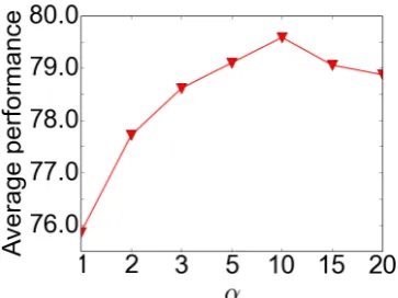
3.2 Effect of Vector Length

How does the length of the overcomplete vector (K) affect performance? We focus here on the Glove vectors, where L = 300, and report av-erage performance across all tasks. We consider

K =αLwhereα∈ {2,3,5,10,15,20}. Figure 2 plots the average performance across tasks against

α. The earlier selection ofK = 3,000(α = 10) gives the best result; gains are monotonic inα to that point and then begin to diminish.

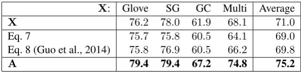
3.3 Alternative Transformations

We consider two alternative transformations. The first preserves the original vector length but

2_{We report correlation on a 100 point scale, so that the}

Vectors SimLex Senti. TREC Sports Comp. Relig._{Corr. Acc. Acc. Acc. Acc. Acc. Acc.}NP Average

Glove XA 3638..99 7781.4.7 81.576.2 9596.3.9 7987.0.7 88.8 82.386.7 77.9 7679.4.2 B 39.7 81.0 81.2 95.7 84.6 87.4 81.6 78.7

SG XA 4143.6.7 8182.7.5 7781..82 9798.2.1 8084..52 8586..5 819 80..61 7978..04

B 42.8 81.6 81.6 95.2 86.5 88.0 82.9 79.8

GC XA 129..07 6873..33 6477..66 7775..01 6860..35 81.0 81.276.0 79.4 6761..92

B 18.7 73.6 79.2 79.7 70.5 79.6 79.4 68.6

Multi XA 2828.7.1 7578.6.5 6379..28 8393..96 7864..23 8481..5 818 79..12 7468..18

B 28.7 77.6 82.0 94.7 81.4 85.6 81.9 75.9

Table 3: Performance comparison of transformed vectors to initial vectorsX. We show sparse over-complete representationsAand also binarized representationsB. Initial vectors are discussed in§A and tasks in§B.

Figure 2: Average performace across all tasks for sparse overcomplete vectors (A) produced by Glove initial vectors, as a function of the ratio of

KtoL.

achieves a binary, sparse vector (B) by applying:

bi,j =

1 ifxi,j >0

0 otherwise (7)

The second transformation was proposed by Guo et al. (2014). Here, the original vector length is also preserved, but sparsity is achieved through:

ai,j =

  

1 ifxi,j ≥M+

−1 ifxi,j ≤M−

0 otherwise (8)

where M+ _(M−_{) is the mean of positive-valued}

(negative-valued) elements of X. These vectors are, obviously, not binary.

We find that on average, across initializing vec-tors and across all tasks that our sparse overcom-plete (A) vectors lead to better performance than either of the alternative transformations.

4 Interpretability

Our hypothesis is that the dimensions of sparse overcomplete vectors are more interpretable than those of dense word vectors. Following Murphy et al. (2012), we use a word intrusion experiment (Chang et al., 2009) to corroborate this hypothesis. In addition, we conduct qualitative analysis of in-terpretability, focusing on individual dimensions. 4.1 Word Intrusion

Word intrusion experiments seek to quantify the extent to which dimensions of a learned word rep-resentation are coherent to humans. In one in-stance of the experiment, a human judge is pre-sented with five words in random order and asked to select the “intruder.” The words are selected by the experimenter by choosing one dimensionj of the learned representation, then ranking the words on that dimension alone. The dimensions are cho-sen in decreasing order of the variance of their values across the vocabulary. Four of the words are the top-ranked words according to j, and the “true” intruder is a word from the bottom half of the list, chosen to be a word that appears in the top 10% of some other dimension. An example of an instance is:

X: Glove SG GC Multi Average

X 76.2 78.0 61.9 68.1 71.0

Eq. 7 75.7 75.8 60.5 64.1 69.0

Eq. 8 (Guo et al., 2014) 75.8 76.9 60.5 66.2 69.8

A 79.4 79.4 67.2 74.8 75.2

Table 4: Average performance across all tasks and vector models using different transformations.

Vectors A1 A2 A3 Avg. IAA κ

X 61 53 56 57 70 0.40

A 71 70 72 71 77 0.45

Table 5: Accuracy of three human annotators on the word intrusion task, along with the average inter-annotator agreement (Artstein and Poesio, 2008) and Fleiss’κ(Davies and Fleiss, 1982).

(The last word is the intruder.)

We formed instances from initializing vectors and from our sparse overcomplete vectors (A). Each of these two combines the four different ini-tializers X. We selected the 25 dimensionsd in each case. Each of the 100 instances per condition (initial vs. sparse overcomplete) was given to three judges.

Results in Table 5 confirm that the sparse over-complete vectors are more interpretable than the dense vectors. The inter-annotator agreement on the sparse vectors increases substantially, from

57% to 71%, and the Fleiss’ κ increases from “fair” to “moderate” agreement (Landis and Koch, 1977).

4.2 Qualitative Evaluation of Interpretability If a vector dimension is interpretable, the top-ranking words for that dimension should display semantic or syntactic groupings. To verify this qualitatively, we select five dimensions with the highest variance of values in initial and sparsi-fied GC vectors. We compare top-ranked words in the dimensions extracted from the two representa-tions. The words are listed in Table 6, a dimension per row. Subjectively, we find the semantic group-ings better in the sparse vectors than in the initial vectors.

Figure 3 visualizes the sparsified GC vectors for six words. The dimensions are sorted by the aver-age value across the three “animal” vectors. The animal-related words use many of the same di-mensions (102 common active didi-mensions out of 500 total); in constrast, the three city names use

X

combat, guard, honor, bow, trim, naval ’ll, could, faced, lacking, seriously, scored see, n’t, recommended, depending, part due, positive, equal, focus, respect, better sergeant, comments, critics, she, videos

A

fracture, breathing, wound, tissue, relief relationships, connections, identity, relations files, bills, titles, collections, poems, songs naval, industrial, technological, marine stadium, belt, championship, toll, ride, coach Table 6: Top-ranked words per dimension for ini-tial and sparsified GC representations. Each line shows words from a different dimension.

mostly distinct vectors.

5 Related Work

V3 79 V3 53 V7 6 V1 86 V3 39 V1 77 V1 14 V3 42 V3 32 V2 70 V2 22 V9 1 V3 03 V4 73 V3 55 V3 58 V1 64 V3 48 V3 24 V1 92 V2 4 V2 81 V8 2 V4 6 V2 77 V4 66 V4 65 V1 28 V1 1 V4 13 V9 8 V1 31 V4 45 V1 99 V4 75 V2 08 V4 31 V2 99 V3 57 V1 49 V8 0 V2 47 V2 31 V4 2 V4 4 V3 76 V1 52 V7 4 V2 54 V1 41 V3 41 V3 49 V2 34 V5 5 V4 77 V2 72 V2 17 V4 57 V5 7 V1 59 V2 23 V3 10 V4 36 V3 25 V2 11 V1 17 V3 60 V4 83 V3 63 V4 39 V4 03 V1 19 V3 29 V8 3 V3 71 V4 24 V1 79 V2 14 V2 68 V3 8 V1 02 V9 3 V8 9 V1 2 V1 72 V1 73 V2 85 V3 44 V7 8 V2 27 V4 26 V4 30 V2 41 V3 84 V4 60 V3 47 V1 71 V2 89 V3

80V8V2V3V5V6V7_V10_V14_V15_V16_V178_V1V19_V20_V21_V22_V25_V26_V28_V29_V30_V31_V32_V335_V3V36_V37_V39_V40_V41_V435_V4V47_V49_V50_V51_V5264_V5V5V58_V59_V60_V63_V645_V6V67_V68_V69_V70_V72_V75_V77_V81_V87_V90_V92_V94_V99

V1 01 V1 03 V1 05 V1 06 V1 08 V1 10 V1 11 V1 16 V1 18 V1 22 V1 23 V1 25 V1 30 V1 32 V1 33 V1 36 V1 37 V1 38 V1 39 V1 40 V1 43 V1 44 V1 47 V1 48 V1 50 V1 55 V1 58 V1 60 V1 62 V1 65 V1 66 V1 67 V1 68 V1 69 V1 70 V1 74 V1 75 V1 78 V1 80 V1 81 V1 82 V1 83 V1 85 V1 88 V1 89 V1 90 V1 91 V1 93 V1 94 V1 95 V1 96 V2 02 V2 03 V2 04 V2 05 V2 12 V2 13 V2 15 V2 18 V2 20 V2 24 V2 26 V2 28 V2 32 V2 33 V2 35 V2 36 V2 38 V2 39 V2 40 V2 42 V2 43 V2 44 V2 48 V2 49 V2 50 V2 51 V2 52 V2 53 V2 55 V2 58 V2 59 V2 60 V2 61 V2 62 V2 63 V2 64 V2 65 V2 66 V2 71 V2 73 V2 74 V2 78 V2 82 V2 84 V2 87 V2 88 V2 90 V2 92 V2 93 V2 94 V2 96 V3 00 V3 02 V3 04 V3 07 V3 08 V3 11 V3 12 V3 13 V3 14 V3 16 V3 17 V3 18 V3 19 V3 20 V3 21 V3 22 V3 23 V3 27 V3 30 V3 31 V3 33 V3 34 V3 36 V3 38 V3 40 V3 43 V3 45 V3 46 V3 52 V3 56 V3 61 V3 62 V3 66 V3 68 V3 69 V3 70 V3 72 V3 73 V3 75 V3 77 V3 78 V3 81 V3 82 V3 83 V3 85 V3 86 V3 87 V3 88 V3 89 V3 90 V3 91 V3 92 V3 94 V3 95 V3 96 V3 98 V3 99 V4 00 V4 01 V4 02 V4 04 V4 05 V4 06 V4 07 V4 08 V4 09 V4 10 V4 12 V4 14 V4 15 V4 16 V4 17 V4 18 V4 19 V4 20 V4 22 V4 23 V4 25 V4 27 V4 28 V4 29 V4 33 V4 34 V4 35 V4 37 V4 41 V4 42 V4 44 V4 46 V4 49 V4 50 V4 51 V4 52 V4 53 V4 55 V4 56 V4 58 V4 59 V4 61 V4 62 V4 63 V4 64 V4 67 V4 68 V4 69 V4 71 V4 72 V4 78 V4 79 V4 80 V4 81 V4 82 V4 84 V4 85 V4 86 V4 88 V4 89 V4 90 V4 91 V4 92 V4 93 V4 94 V4 95 V4 97 V4 99 V5 00 V5 01 V4 87 V2 00 V3 26V4 V1 21 V2 67 V2 30 V4 38 V1 34 V9 7 V1 04 V3 51 V2 19 V1 3 V8 8 V1 29 V2 86 V2 29 V3 50 V9 6 V1 07 V1 53 V1 45 V1 54 V3 4 V3 01 V3 74 V1 09 V3 97 V1 56 V1 61 V2 97 V1 15 V1 51 V2 45 V4 47 V5 3 V3 37 V7 9 V4 48 V2 83 V4 43 V2 01 V3 93 V3 65 V4 8 V1 26 V2 57 V2 46 V2 95 V1 20 V3 67 V2 7 V1 84 V2 09 V3 06 V2 69 V1 24 V4 70 V1 12 V1 87 V6 2 V4 74 V3 54 V4 54 V2 79 V1 46 V2 75 V2 21 V2 07 V7 1 V3 35 V7 3 V8 5 V4 40 V9 5 V2 3 V2 25 V4 11 V3 28 V3 05 V1 98 V1 63V9 V1 35 V3 15 V1 42 V4 98 V2 91 V8 6 V4 76 V2 10 V3 59 V8 4 V1 00 V3 09 V1 76 V2 16 V4 32 V2 06 V4 21 V2 76 V2 37 V6 1 V1 57 V3 64 V1 27 V6 6 V2 56 V2 80 V1 13 V2 98 V1 97 V4 96 boston seattle chicago dog horse fish

Figure 3: Visualization of sparsified GC vectors. Negative values are red, positive values are blue, zeroes are white.

6 Conclusion

We have presented a method that converts word vectors obtained using any state-of-the-art word vector model into sparse and optionally binary word vectors. These transformed vectors appear to come closer to features used in NLP tasks and out-perform the original vectors from which they are derived on a suite of semantics and syntactic eval-uation benchmarks. We also find that the sparse vectors are more interpretable than the dense vec-tors by humans according to a word intrusion de-tection test.

Acknowledgments

We thank Alona Fyshe for discussions on vec-tor interpretability and three anonymous review-ers for their feedback. This research was sup-ported in part by the National Science Foundation through grant IIS-1251131 and the Defense Ad-vanced Research Projects Agency through grant FA87501420244. This work was supported in part by the U.S. Army Research Laboratory and the U.S. Army Research Office under contract/grant number W911NF-10-1-0533.

A Initial Vector Representations (X) Our experiments consider four publicly available collections of pre-trained word vectors. They vary in the amount of data used and the estimation method.

Glove. Global vectors for word representations (Pennington et al., 2014) are trained on aggregated global word-word co-occurrence statistics from a corpus. These vectors were trained on 6 billion words from Wikipedia and English Gigaword and are of length 300.3

3_{http://www-nlp.stanford.edu/projects/}

glove/

Skip-Gram (SG). The word2vec tool (Mikolov et al., 2013) is fast and widely-used. In this model, each word’s Huffman code is used as an input to a log-linear classifier with a continuous projection layer and words within a given context window are predicted. These vectors were trained on 100 bil-lion words of Google news data and are of length 300.4

Global Context (GC). These vectors are learned using a recursive neural network that incorporates both local and global (document-level) context features (Huang et al., 2012). These vectors were trained on the first 1 billion words of English Wikipedia and are of length 50.5

Multilingual (Multi). Faruqui and Dyer (2014) learned vectors by first performing SVD on text in different languages, then applying canonical correlation analysis on pairs of vectors for words that align in parallel corpora. These vectors were trained on WMT-2011 news corpus containing 360 million words and are of length 48.6

B Evaluation Benchmarks

Our comparisons of word vector quality consider five benchmark tasks. We now describe the differ-ent evaluation benchmarks for word vectors.

Word Similarity. We evaluate our word repre-sentations on two word similarity tasks. The first is the WS-353 dataset (Finkelstein et al., 2001), which contains 353 pairs of English words that have been assigned similarity ratings by humans. This dataset is used to tune sparse vector learning hyperparameters (§2.5), while the remaining of the tasks discussed in this section are completely held out.

4_{https://code.google.com/p/word2vec} 5_{http://nlp.stanford.edu/˜socherr/}

ACL2012_wordVectorsTextFile.zip

A more recent dataset, SimLex-999 (Hill et al., 2014), has been constructed to specifically focus on similarity (rather than relatedness). It con-tains a balanced set of noun, verb, and adjective pairs. We calculate cosine similarity between the vectors of two words forming a test item and re-port Spearman’s rank correlation coefficient (My-ers and Well, 1995) between the rankings pro-duced by our model against the human rankings.

Sentiment Analysis (Senti). Socher et al. (2013) created a treebank of sentences anno-tated with fine-grained sentiment labels on phrases and sentences from movie review excerpts. The coarse-grained treebank of positive and negative classes has been split into training, development, and test datasets containing 6,920, 872, and 1,821 sentences, respectively. We use average of the word vectors of a given sentence as feature for classification. The classifier is tuned on the dev. set and accuracy is reported on the test set.

Question Classification (TREC). As an aid to question answering, a question may be classi-fied as belonging to one of many question types. The TREC questions dataset involves six differ-ent question types, e.g., whether the question is about a location, about a person, or about some nu-meric information (Li and Roth, 2002). The train-ing dataset consists of 5,452 labeled questions, and the test dataset consists of 500 questions. An av-erage of the word vectors of the input question is used as features and accuracy is reported on the test set.

20 Newsgroup Dataset. We consider three bi-nary categorization tasks from the 20 News-groups dataset.7 _{Each task involves} categoriz-ing a document accordcategoriz-ing to two related cate-gories with training/dev./test split in accordance with Yogatama and Smith (2014): (1) Sports: baseball vs. hockey (958/239/796) (2) Comp.: IBM vs. Mac (929/239/777) (3) Religion: atheism vs. christian (870/209/717). We use average of the word vectors of a given sentence as features. The classifier is tuned on the dev. set and accuracy is reported on the test set.

NP bracketing (NP). Lazaridou et al. (2013) constructed a dataset from the Penn Treebank (Marcus et al., 1993) of noun phrases (NP) of

7_{http://qwone.com/˜jason/20Newsgroups}

length three words, where the first can be an ad-jective or a noun and the other two are nouns. The task is to predict the correct bracketing in the parse tree for a given noun phrase. For example, local (phone company) and (blood pressure) medicine

exhibitrightandleftbracketing, respectively. We append the word vectors of the three words in the NP in order and use them as features for binary classification. The dataset contains 2,227 noun phrases split into 10 folds. The classifier is tuned on the first fold and cross-validation accuracy is reported on the remaining nine folds.

References

Faiz A. Al-Khayyal and James E. Falk. 1983. Jointly constrained biconvex programming.Mathematics of Operations Research, pages 273–286.

Ron Artstein and Massimo Poesio. 2008. Inter-coder agreement for computational linguistics. Computa-tional Linguistics, 34(4):555–596.

Collin F. Baker, Charles J. Fillmore, and John B. Lowe. 1998. The Berkeley FrameNet project. InProc. of ACL.

Mohit Bansal, Kevin Gimpel, and Karen Livescu. 2014. Tailoring continuous word representations for dependency parsing. InProc. of ACL.

Yoshua Bengio, Aaron Courville, and Pascal Vincent. 2013. Representation learning: A review and new perspectives. IEEE Transactions on Pattern Analy-sis and Machine Intelligence, 35(8):1798–1828.

Jonathan Chang, Sean Gerrish, Chong Wang, Jordan L. Boyd-Graber, and David M. Blei. 2009. Reading tea leaves: How humans interpret topic models. In

NIPS.

Andrzej Cichocki, Rafal Zdunek, Anh Huy Phan, and Shun-ichi Amari. 2009. Nonnegative Matrix and Tensor Factorizations: Applications to Exploratory Multi-way Data Analysis and Blind Source Separa-tion. John Wiley & Sons.

Mark Davies and Joseph L Fleiss. 1982. Measuring agreement for multinomial data. Biometrics, pages 1047–1051.

David L. Donoho, Michael Elad, and Vladimir N. Temlyakov. 2006. Stable recovery of sparse over-complete representations in the presence of noise.

IEEE Transactions on Information Theory, 52(1).

John C. Duchi, Alekh Agarwal, and Martin J. Wain-wright. 2012. Dual averaging for distributed opti-mization: Convergence analysis and network scal-ing. IEEE Transactions on Automatic Control, 57(3):592–606.

Manaal Faruqui and Chris Dyer. 2014. Improving vector space word representations using multilingual correlation. InProc. of EACL.

Manaal Faruqui, Jesse Dodge, Sujay K. Jauhar, Chris Dyer, Eduard Hovy, and Noah A. Smith. 2015. Retrofitting word vectors to semantic lexicons. In

Proc. of NAACL.

Lev Finkelstein, Evgeniy Gabrilovich, Yossi Matias, Ehud Rivlin, Zach Solan, Gadi Wolfman, and Ey-tan Ruppin. 2001. Placing search in context: the concept revisited. InProc. of WWW.

Jerome Friedman, Trevor Hastie, and Robert Tibshi-rani. 2008. Sparse inverse covariance estimation with the graphical lasso. Biostatistics, 9(3):432– 441.

Alona Fyshe, Partha P. Talukdar, Brian Murphy, and Tom M. Mitchell. 2014. Interpretable semantic vec-tors from a joint model of brain- and text- based meaning. InProc. of ACL.

Alona Fyshe, Leila Wehbe, Partha P. Talukdar, Brian Murphy, and Tom M. Mitchell. 2015. A composi-tional and interpretable semantic space. InProc. of NAACL.

Kuzman Ganchev, Ben Taskar, Fernando Pereira, and Jo˜ao Gama. 2009. Posterior vs. parameter sparsity in latent variable models. InNIPS.

Xavier Glorot, Antoine Bordes, and Yoshua Bengio. 2011. Domain adaptation for large-scale sentiment classification: A deep learning approach. InProc. of ICML.

Joshua Goodman. 2004. Exponential priors for maxi-mum entropy models. InProc. of NAACL.

E. Grefenstette. 2013. Towards a formal distributional semantics: Simulating logical calculi with tensors. arXiv:1304.5823.

Jiang Guo, Wanxiang Che, Haifeng Wang, and Ting Liu. 2014. Revisiting embedding features for sim-ple semi-supervised learning. InProc. of EMNLP.

Georg Heigold, Erik McDermott, Vincent Vanhoucke, Andrew Senior, and Michiel Bacchiani. 2014. Asynchronous stochastic optimization for sequence training of deep neural networks. In Proc. of ICASSP.

Felix Hill, Roi Reichart, and Anna Korhonen. 2014. Simlex-999: Evaluating semantic models with (gen-uine) similarity estimation. CoRR, abs/1408.3456.

Patrik O. Hoyer. 2002. Non-negative sparse coding. In

Neural Networks for Signal Processing, 2002. Proc. of IEEE Workshop on.

Eric H. Huang, Richard Socher, Christopher D. Man-ning, and Andrew Y. Ng. 2012. Improving word representations via global context and multiple word prototypes. InProc. of ACL.

Jun’ichi Kazama and Jun’ichi Tsujii. 2003. Evaluation and extension of maximum entropy models with in-equality constraints. InProc. of EMNLP.

Douwe Kiela and Stephen Clark. 2013. Detecting compositionality of multi-word expressions using nearest neighbours in vector space models. InProc. of EMNLP.

J. Richard Landis and Gary G. Koch. 1977. The mea-surement of observer agreement for categorical data.

Biometrics, 33(1):159–174.

Angeliki Lazaridou, Eva Maria Vecchi, and Marco Baroni. 2013. Fish transporters and miracle homes: How compositional distributional semantics can help NP parsing. InProc. of EMNLP.

Daniel D. Lee and H. Sebastian Seung. 1999. Learning the parts of objects by non-negative matrix factoriza-tion. Nature, 401(6755):788–791.

Honglak Lee, Alexis Battle, Rajat Raina, and An-drew Y. Ng. 2006. Efficient sparse coding algo-rithms. InNIPS.

Honglak Lee, Rajat Raina, Alex Teichman, and An-drew Y. Ng. 2009. Exponential family sparse cod-ing with application to self-taught learncod-ing. InProc. of IJCAI.

Beth Levin. 1993. English Verb Classes and Alter-nations: A Preliminary Investigation. University of Chicago Press.

Michael Lewicki and Terrence Sejnowski. 2000. Learning overcomplete representations. Neural Computation, 12(2):337–365.

Mike Lewis and Mark Steedman. 2013. Combined distributional and logical semantics. Transactions of the ACL, 1:179–192.

Mike Lewis and Mark Steedman. 2014. Combining formal and distributional models of temporal and in-tensional semantics. InProc. of ACL.

Xin Li and Dan Roth. 2002. Learning question classi-fiers. InProc. of COLING.

Weixiang Liu, Nanning Zheng, and Xiaofeng Lu. 2003. Non-negative matrix factorization for visual coding. InProc. of ICASSP.

Andr´e F. T. Martins, Noah A. Smith, Pedro M. Q. Aguiar, and M´ario A. T. Figueiredo. 2011. Struc-tured sparsity in strucStruc-tured prediction. InProc. of EMNLP.

Tomas Mikolov, Kai Chen, Greg Corrado, and Jeffrey Dean. 2013. Efficient estimation of word represen-tations in vector space.

George A. Miller. 1995. WordNet: a lexical database for English. Communications of the ACM, 38(11):39–41.

Brian Murphy, Partha Talukdar, and Tom Mitchell. 2012. Learning effective and interpretable seman-tic models using non-negative sparse embedding. In

Proc. of COLING.

Jerome L. Myers and Arnold D. Well. 1995. Research Design & Statistical Analysis. Routledge.

Bruno A. Olshausen and David J. Field. 1997. Sparse coding with an overcomplete basis set: A strategy employed by v1? Vision Research, 37(23):3311 – 3325.

Denis Paperno, Nghia The Pham, and Marco Baroni. 2014. A practical and linguistically-motivated ap-proach to compositional distributional semantics. In

Proc. of ACL.

Michael Paul and Mark Dredze. 2012. Factorial LDA: Sparse multi-dimensional text models. InNIPS. Jeffrey Pennington, Richard Socher, and

Christo-pher D. Manning. 2014. Glove: Global vectors for word representation. InProc. of EMNLP.

Karin Kipper Schuler. 2005. Verbnet: A Broad-coverage, Comprehensive Verb Lexicon. Ph.D. the-sis, University of Pennsylvania.

Richard Socher, Alex Perelygin, Jean Wu, Jason Chuang, Christopher D. Manning, Andrew Y. Ng, and Christopher Potts. 2013. Recursive deep mod-els for semantic compositionality over a sentiment treebank. InProc. of EMNLP.

Kristina Toutanova and Mark Johnson. 2007. A bayesian lda-based model for semi-supervised part-of-speech tagging. InNIPS.

Peter D. Turney and Patrick Pantel. 2010. From fre-quency to meaning : Vector space models of seman-tics. JAIR, 37(1):141–188.

Peter D. Turney. 2001. Mining the web for synonyms: PMI-IR versus LSA on TOEFL. InProc. of ECML. Eva Maria Vecchi, Roberto Zamparelli, and Marco Ba-roni. 2013. Studying the recursive behaviour of adjectival modification with compositional distribu-tional semantics. InProc. of EMNLP.

Lin Xiao. 2009. Dual averaging methods for regular-ized stochastic learning and online optimization. In

NIPS.

Chang Xu, Yalong Bai, Jiang Bian, Bin Gao, Gang Wang, Xiaoguang Liu, and Tie-Yan Liu. 2014. Rc-net: A general framework for incorporating knowl-edge into word representations. InProc. of CIKM. Dani Yogatama and Noah A Smith. 2014. Linguistic

structured sparsity in text categorization. InProc. of ACL.

Mo Yu and Mark Dredze. 2014. Improving lexical embeddings with semantic knowledge. In Proc. of ACL.