Memory-Optimized Software Synthesis
from Dataflow Program Graphs
with Large Size Data Samples
Hyunok Oh
The School of Electrical Engineering and Computer Science, Seoul National University, Seoul 151-742, Korea Email:[email protected]
Soonhoi Ha
The School of Electrical Engineering and Computer Science, Seoul National University, Seoul 151-742, Korea Email:[email protected]
Received 28 February 2002 and in revised form 15 October 2002
In multimedia and graphics applications, data samples of nonprimitive type require significant amount of buffer memory. This paper addresses the problem of minimizing the buffer memory requirement for such applications in embedded software synthesis from graphical dataflow programs based on the synchronous dataflow (SDF) model with the given execution order of nodes. We propose a memory minimization technique that separates global memory buffers from local pointer buffers: the global buffers store live data samples and the local buffers store the pointers to the global buffer entries. The proposed algorithm reduces 67% memory for a JPEG encoder, 40% for an H.263 encoder compared with unshared versions, and 22% compared with the previous sharing algorithm for the H.263 encoder. Through extensive buffer sharing optimization, we believe that automatic software synthesis from dataflow program graphs achieves the comparable code quality with the manually optimized code in terms of memory requirement.
Keywords and phrases:software synthesis, memory optimization, multimedia, dataflow.
1. INTRODUCTION
Reducing the size of memory is an important objective in embedded system design since an embedded system has tight area and power budgets. Therefore, application designers usually spend significant amount of code development time to optimize the memory requirement.
On the other hand, as system complexity increases and fast design turn-around time becomes important, it attracts more attention to use high-level software design methodol-ogy: automatic code generation from block diagram specifi-cation. COSSAP [1], GRAPE [2], and Ptolemy [3] are well-known design environments, especially for digital signal pro-cessing applications, with automatic code synthesis facility from graphical dataflow programs.
In a hierarchical dataflow program graph, a node, or a block, represents a function that transforms input data streams into output streams. The functionality of an atomic node is described in a high-level language such as C or VHDL. An arc represents a channel that carries streams of data samples from the source node to the destination node. The number of samples produced (or consumed) per node
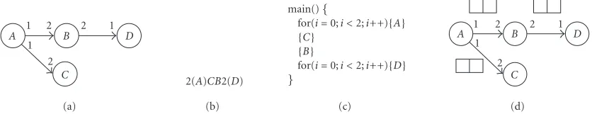
firing is called the output (or the input) sample rate of the node. In case the number of samples consumed or produced on each arc is statically determined and can be any integer, the graph is called a synchronous dataflow graph (SDF) [4] which is widely adopted in aforementioned design environ-ments. We illustrate an example of SDF graph inFigure 1a. Each arc is annotated with the number of samples consumed or produced per node execution. In this paper, we are con-cerned with memory optimized software synthesis from SDF graphs though the proposed techniques can be easily ex-tended to other SDF extensions.
C B
A D
1 2
1 2 2 1
(a)
2(A)CB2(D) (b)
main(){
for(i=0;i <2;i++){A} {C}
{B}
for(i=0;i <2;i++){D} }
(c)
C B
A D
1 2
1 2 2 1
(d)
Figure1: (a) SDF graph example, (b) a scheduling result, (c) a code template, and (d) a buffer allocation.
DCT−1 8×8 Zigzag−1 8×8
Q−1 8×8 Q 8×8 Zigzag 8×8 DCT
a b c d e
A B
Figure2: Image processing example.
between the source and the destination blocks. The number of allocated buffer entries should be no less than the maxi-mum number of samples accumulated on the arc at runtime. After block Ais executed twice, two data samples are pro-duced on each output arc as explicitly depicted inFigure 1d. We define a buffer allocated on each arc as a local buffer that is used for data transfer between two associated blocks. If the data samples are of primitive types, the local buffers store data values and the generated code defines a local buffer with an array of primitive type data.
Required memory spaces in the synthesized code con-sist of code segments and data segments. The latter stores constants and parameters as well as data samples. We regard memory space for data samples as buffer memory, or shortly buffer, in this paper.
There are several classes of applications that deal with nonprimitive data types. The typical data type of an image processing application is a matrix of fixed block size as il-lustrated in Figure 2. Graphic applications usually need to deal with structure-type data samples that contain informa-tion on vertex coordinates, viewpoints, light sources, and so on. Networked multimedia applications exchange pack-ets of data samples between blocks. In those applications, the buffer requirements are likely to be more significant than others. For example, the code size of H.263 encoder [5] is about 100 K bytes but the buffer size is more than 300 K bytes.
Since the buffer requirement of an SDF graph depends on the execution order of nodes, there have been several ap-proaches [6, 7, 8] to take the buffer size minimization as one of the scheduling objectives. However, they do not con-sider either buffer sharing possibilities nor nonprimitive data types. Finding out an optimal schedule for minimum buffer requirements considering both is a future research topic.In this paper, instead, we propose a buffer sharing technique for nonprimitive type data samples to minimize the buffer mem-ory requirement assuming that the execution order of nodes is
already determined at compile time. Thus, this work is com-plementary to existent scheduling algorithms to further re-duce the buffer requirement.
Figure 2demonstrates a simple example where we can re-duce the significant amount of buffer memory by sharing buffers. Without buffer sharing, five local buffers of size 64 (= 8×8) are needed. On the other hand, only two buffers are needed if buffer sharing is used so thata,c, andebuffers share bufferA, andbanddbuffers share bufferB. Such shar-ing decision can be made at compile time through lifetime analysis of data samples, which is a well-known compilation technique.
A key difference between the proposed technique and the previous approaches is that we separate the local pointer buffers from global data buffers explicitly in the synthesized code. In Figure 2, we use five local pointer buffers and two
global buffers. This separation provides more memory shar-ing chances when the number of local buffer entries becomes more than one. If the local buffer size becomes one after buffer optimization, no separation is needed. We examine
Figure 3a which illustrates a simplified version of an H.263 encoder algorithm where “ME” node indicates a motion esti-mation block, “Trans” is a transform coding block which per-forms DCT and Quantization, and “InvTrans” perper-forms in-verse transform coding and image reconstruction. Each sam-ple between nodes is a frame of 176×144 byte size which is large enough to ignore local buffer size. The diamond sym-bol on the arc between ME and InvTrans denotes an initial data sample, which is the previous frame in this example. If we do not separate local buffers from global buffers, then we need three frame buffers as shown inFigure 3bsince buffers aandcoverlap their lifetimes at ME,aandbat Trans, andb andcat InvTrans. Even though two frames are sufficient for this graph, we cannot share any buffer without separation of local buffers and global buffers. In fact, we can use only two frame buffers if we use separate local pointer buffers.
1
Figure3: (a) Simplified H.263 encoder in which a diamond between InvTrans and ME indicates an initial sample delay, (b) and (c) a minimum buffer allocation without and with separation of global buffers and local buffers, respectively.
C
Figure4: (a) An example of SDF graph with an initial delay betweenBandCillustrated by a diamond, (b) the sample lifetime chart, (c) a global buffer lifetime chart, and (d) a local buffer lifetime chart.
buffers, and the mapping of local buffers to global buffers. The detailed algorithm and code synthesis techniques will be explained inSection 4.
It is NP-hard to determine the optimal local buffer, global buffer sizes, and their mappings in general cases where there are feedback structures in the graph topology. The problem becomes harder if we consider buffer sharing among different size data samples. Therefore, we devise a heuristic that focuses on global buffer minimization first and applies an optimal algorithm next to find the minimum local pointer buffer sizes and to map the local pointer buffers to the min-imum global buffers. The proposed heuristic results in less than 5% overhead than an optimal solution on average.
In Section 2, we define a new buffer sharing problem for nonprimitive data types, and survey the previous works briefly. The overview of the proposed technique is presented in Section 3. Section 4 explains how to minimize the size of local buffers and their mappings to the minimum global buffers assuming that all data samples have the same size. In
Section 5, we extend the technique to the case where data samples have the different sizes. Graphs with initial sam-ples are discussed inSection 6. Finally, we present some ex-perimental results in Section 7, and make conclusions in
Section 8.
2. PROBLEM STATEMENT AND PREVIOUS WORKS In the proposed technique, global buffers store the live data samples of nonprimitive type while the local pointer buffers
store the pointers for the global buffer entries. Since multiple data samples can share the buffer space as long as their life-times do not overlap, we should examine the lifelife-times of data samples. We denotes(a, k) as thekth stored sample on arca and TNSE(a) as the total number of samples exchanged dur-ing an iteration cycle. Consider an example ofFigure 4awith the associated schedule. TNSE(a) becomes 2 and two sam-ples,s(a,1) ands(a,2), are produced and consumed on arc a. Arcbhas an initial samples(b,1) and two more samples, s(b,2) ands(b,3), during an iteration cycle.
The lifetimes of data samples are displayed in the sam-ple lifetime chartas shown inFigure 4b, where the horizontal axis indicates the abstract notion of time: each invocation of a node is considered to be one unit of time. The vertical axis in-dicates the memory size and each rectangle denotes the life-time interval of a data sample. Note that each sample lifelife-time defines a single time interval whose start time is the invoca-tion time of the source block and the stop time is the comple-tion time of the destinacomple-tion block. For example, the lifetime interval of samples(b,2) is [B1, C1]. We take special care of initial samples. The lifetime of samples(b,1) is carried for-ward from the last iteration cycle while that of samples(b,3) is carried forward to the next iteration cycle. We denote the former-type interval as atail lifetime interval, or shortly a tail interval, and the latter as ahead lifetime interval, or a head in-terval. In fact, samples(b,3) at the current iteration cycle be-comess(b,1) at the next iteration cycle. To distinguish itera-tion cycles, we usesk(b,2) to indicate samples(b,2) at thekth
And the sample lifetime that spans multiple iteration cycles is defined as amulticycle lifetime. Note that the sample lifetime chart is determined from the schedule.
From the sample lifetime chart, it is obvious that the minimum size of global buffer memory is the maximum of the total memory requirements of live data samples over time. We summarize this fact as the following lemma with-out proof.
Lemma 1. The minimum size of global buffer memory is equal to the maximum total size of live data samples at any instance during an iteration cycle.
We map the sample lifetimes to the global buffers: an example is shown inFigure 4cwhereg(k) indicates thekth global buffer. In case all data types have the same size, an in-terval scheduling algorithm can successfully map the sample lifetimes to the minimum size of global buffer memory.
Sample lifetime is distinguished from local buffer lifetime since a local buffer may store multiple samples during an iter-ation cycle. Consider an example ofFigure 4awhere the local buffer sizes of arcsaandbare set to be 1 and 2, respectively. We denoteB(a, k) as thekth local buffer entry on arca. Then, thelocal buffer lifetime chartbecomes as drawn inFigure 4d. BufferB(a,1) stores two samples,s(a,1) ands(a,2), to have multiple lifetime intervals during an iteration cycle. Now, we state the problem this paper aims to solve as follows.
Problem 1. Determine LB(g, s(g)) and GB(g, s(g)) in order to minimize the sum of them, where LB(g, s(g)) is the sum of local buffer sizes on all arcs and GB(g, s(g)) is the global buffer size with a given graphgand a given schedules(g).
Since the simpler problems are NP-hard, this problem is NP-hard, too. Consider a special case when all samples have the same type or the same size. For a given local buffer size, determining the minimum global buffer size is difficult if a local buffer may have multiple lifetime intervals, which is stated in the following theorem.
Theorem 1. If the lifetime of a local buffer may have multi-ple lifetime intervals and all data types have the same size, the decision problem whether there exists a mapping from a given number of local buffers to a given number of global buffers is NP-hard.
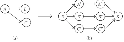
Proof. We will prove this theorem by showing that the graph coloring problem can be reduced to this mapping problem. Consider a graph G(V, E) whereV is a vertex set andE is an edge set. A simple example graph is shown inFigure 5a. We associate a new graph G (Figure 5b) where a pair of nodes are created for each vertex of graphGand connected to the dummy source node S and the dummy sink node K of the graphG. In other words, a vertex in graph Gis mapped to a local buffer in graph G. The next step is to map an arc of graphGto a schedule sequence in graphG. For instance, an arcABin graph Gis mapped to a sched-ule segment (ABAB) to enforce that two local buffers on
K B B
S A
C
A
C B
C A
(a) (b)
Figure5: (a) An example instance of graph coloring problem, and (b) the mapped graph for the proof ofTheorem 1.
arcs AA andBB may not be shared. As we traverse all arcs of graphG, we generate a valid schedule of graphG. Traversing arcsABandACin graphGgenerates a schedule: S(ABAB)(ACAC)K. From this schedule, we find out that the buffer lifetime on arcAAconsists of two intervals. The constraint that two adjacent nodes in Gmay not have the same color is translated to the constraint that two local buffers may not be shared inG. Therefore, the graph color-ing problem for graphGis reduced to the mapping problem for graphG.
The register allocation problem in traditional compilers is to share the memory space for the variables of nonover-lapped lifetimes [9]. If the variable sizes are not uniform, the allocation problem, known as the dynamic storage allocation problem [10,11], isNP-complete. In our context, this prob-lem is equivalent to minimize the global buffer memory ig-noring the local buffer sizes and mapping problems.
De Greef et al. [12] presented a systematic procedure to share arrays for multimedia applications in a synthesis tool called ATOMIUM. They analyze lifetimes of array variables during a single iteration trace of a C program and do not con-sider the case where lifetimes span multiple iteration cycles. If the program is retimed, some variables can be live longer than a single iteration cycle. Another extension we make in the proposed approach is that we consider each array element separately for sharing decision when each array element is of nonprimitive type.
Recently, Murthy and Bhattacharyya [13] proposed a scheduling technique for SDF graphs to optimize the lo-cal memory size by buffer sharing. Since they assume only primitive type data, their sharing decision considers array variables as a whole. However, their research result is com-plementary to our work since the schedule reduces the num-ber of live data samples at runtime, which reduces the global memory size in our framework. They compared their re-search work with Ritz et al.’s [14] whose schedule pat-tern does not allow nested loop structure. They showed that nested loop structure may significantly reduce the local memory size.
1:Uis a set of sample lifetimes;Pis an empty global buffer lifetime chart. 2: While (Uis not empty){
3: Take out a sample lifetimexwith the earliest start time fromU.
4: Find out a global buffer whose lifetime ends earlier than the start time ofx. 5: Priority is given to the buffer that stores samples on the same arc if exists. 6: If no such global buffer exists inP, create another global buffer.
7: Mapxto the selected global buffer 8:}
Figure6: Interval scheduling algorithm.
B A
2 3
a
2(A)BAB
(a)
B2
A3
B1
A2
A1 Samples
s(a,1)
s(a,2)
s(a,3)
s(a,4)
s(a,5)
s(a,6)
(b)
B2
A3
B1
A2
A1 Global
buffer
s(a,1) s(a,6)
s(a,2) s(a,5)
s(a,3)
s(a,4)
g(1)
g(2)
g(3)
g(4)
(c)
B A
B(1)B(2)B(3)B(4) Global
buffer g(1) g(2)g(3) g(4) (d)
Figure7: (a) An SDF subgraph with a given schedule, (b) the sample lifetime chart, (c) the global buffer lifetime chart, and (d) local buffer
allocation and mapping.
3. PROPOSED TECHNIQUE
In this section, we sketch the proposed heuristic for the prob-lem stated in the previous section. Since the size of nonprimi-tive data type is usually much larger than that of pointer type in multimedia applications of interest, reducing the global buffer size is more important than reducing the local pointer buffers. Therefore, our heuristic consists of two phases: the first phase is to map the sample lifetimes within an iteration cycle into the minimum number of global buffers ignoring local buffer sizes, and the second phase is to determine the minimum local buffer sizes and to map the local buffers to the given global buffers.
3.1. Global buffer minimization
Recall that a sample lifetime has a single interval within an iteration cycle. When all samples have the same data size, the interval scheduling algorithm is known to be an optimal algorithm [15] to find the minimum global buffer size. We summarize the interval scheduling algorithm inFigure 6.
Consider an example of Figure 4a whose global buffer
lifetime chart is displayed inFigure 4c. After sampless(a,1), s(b,1), and s(b,2) are mapped into three global buffers, s(a,2) can be mapped to all three buffers. Among the can-didate global buffers, we select one that already storess(a,1) according to the policy of line 5 ofFigure 6. The reason of this priority selection is to minimize the local buffer sizes, which will be discussed in the next section.
When the data samples have different sizes, this mapping problem becomes NP-hard since a special case can be re-duced to 3-partition problem [10]. Therefore, we develop a heuristic, which will be discussed inSection 5.
3.2. Local buffer size determination
The global buffer minimization algorithm in the previous phase runs for one iteration cycle while the graph will be ex-ecuted repeatedly. The next phase is to determine the mini-mum local buffer sizes that are necessary to store the point-ers of data samples mapped to the global buffpoint-ers. Initially we assign a separate local buffer to each live sample during an it-eration cycle. Then, the local buffer size on each arc becomes the total number of live samples within an iteration cycle: each sample occupies a separate local buffer. InFigure 4a, for instance, two local buffers are allocated on arcawhile three local buffers on arcb.
What is the optimal local buffer size? The answer depends on when we set the pointer values, or when webindthe local buffers to the global buffers. If binding is performed statically at compile time, we call it staticbinding. If binding can be changed at runtime, it is calleddynamicbinding. In general, the dynamic binding can reduce the local buffer size signifi-cantly with small runtime overhead of global buffer manage-ment.
3.2.1 Dynamic binding strategy
samples,s(a,1) ands(a,5), which are unfortunately mapped to different global buffers. It means that the pointer value of local bufferB(a,1) should be set tog(1) at the first invocation of nodeAbut tog(2) at the third invocation, dynamically. We repeat this pointer assignment at every iteration cycle at runtime.
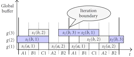
If there are initial samples on an arc, care should be taken to compute the repetition period of pointer assignment. Arc bofFigure 4ahas an initial sample and needs only two local buffers since there are at most two live samples at the same time. Unlike the previous example of Figure 7, the global buffer lifetime chart may not repeat itself at the next itera-tion cycle. The lifetime patterns of local buffersB(b,1) and B(b,2) are interchanged at the next iteration cycle as shown inFigure 8. In other words, the repetition periods of pointer assignment for arcs with initial samples may span multiple iteration cycles.Section 4is devoted to computing the repe-tition period of pointer assignment for the arcs with initial samples.
Suppose an arc a has M local buffers. Since the local buffers are accessed sequentially, each local buffer entry has at mostTNSE(a)/Msamples and the pointer to samples(a, k) is stored inB(a, kmodM). After the first phase is completed, we examine the mapping results of the allocated sample in a local buffer to the global buffers at the code generation stage. If the mapping result of the current sample is changed from the previous one, a code segment is inserted automatically to alter the pointer value at the current schedule instance. Note that it incurs both memory overhead of code insertion and time overhead of runtime mapping.
3.2.2 Static binding strategy
If we use static binding, we may not change the pointer values of local buffers at runtime. It means that all allocated samples to a local buffer should be mapped to the same global buffer. For example ofFigure 7, we need six local buffers for static binding: two more buffers than the dynamic binding case sinces(a,1) ands(a,5) are not mapped to the same global buffer. On the other hand, arcaofFigure 4needs only one local buffer for static binding since two allocated samples are mapped to the same global buffer. How many buffers do we need for arcbofFigure 4for static binding?
To answer this question, we extend the global buffer time chart over multiple iteration cycles until the sample life-time patterns on the arc become periodic. We need to extend the lifetime chart over two iteration cycles as displayed in
Figure 8. Note that the head interval ofs2(b,3) is connected
to the tail interval of s3(b,1) in the next repetition period.
Therefore, four live samples are involved in the repetition pe-riod that consists of two iteration cycles. The problem is to find the minimum local buffer sizeMsuch that all allocated samples on each local buffer are mapped to the same global buffer. The minimum number is four in this example since s3(b,1) can be placed at the same local buffer ass1(b,1).
How many iteration cycles should be extended is an equivalent problem to computing the repetition period of pointer assignment for dynamic binding case. We refer to the next section for detailed discussion.
t
Figure8: The global buffer lifetime chart spanning two iteration
cycles for the example ofFigure 4.
4. REPETITION PERIOD OF SAMPLE LIFETIME PATTERNS
Initial samples may make the repetition period of the sample lifetime chart longer than a single iteration cycle since their lifetimes may span to multiple cycles. In this section, we show how to compute the repetition period of sample lifetime pat-terns to determine the periodic pointer assignment for dy-namic binding or to determine the minimum size of local buffers for static binding. For simplicity, we assume that all samples have the same size in this section. This assumption will be released inSection 5.
First, we compute the iteration length of a sample life-time. Suppose dinitial samples stay alive on an arc andN samples are newly produced for each iteration cycle. Then,N samples on the arc are consumed from the destination node. If dis greater thanN, the newly produced samples all live longer than an iteration cycle. Otherwise,N−dnewly cre-ated samples are consumed during the same iteration cycle while dsamples live longer. We summarize this fact in the following lemma.
Letpbe the number of iteration cycles in which a sample lifetime interval lies.Figure 9illustrates two patterns that a sample lifetime interval can have in a global lifetime chart. A sample starts its lifetime at the first iteration cycle with a head interval and ends its lifetime at the pth iteration with a tail interval. Note that the tail interval at the pth iteration also appears at the first iteration cycle. The first pattern, as shown inFigure 9a, occurs when the tail interval is mapped to the same global buffer as the head interval. The interval mapping pattern repeats every p−1 iteration cycles in this case.
Tail interval
p−1 Head interval Tail Global buffer
Iterations 1 2 · · · p
(a)
Tail interval
p
Global buffer
1 2 · · · p p+ 1
(b)
Figure9: Illustration of a sample lifetime interval: (a) when the tail interval is mapped to the same global buffer as the head interval, and
(b) when the tail interval is mapped to a different global buffer and there is no chained multicycle sample lifetime interval.
k+p1+ · · ·+pn
k+p1+ · · ·+pn−1
k+p1+p2
k+p1
k
Global buffer
tn−1 hn
t1 h2
tn h1 · · ·
t1 h2 · · ·
t2 h3 · · ·
tn−1 hn · · ·
tn h1
t1 h2
tn−1 hn
(a)
k+ 2 +p1 +· · ·+pn
k+ 1 +p1 +· · ·+pn
k+ 1 +p1 +· · ·+pn−1
k+ 1+
p1+p2
k+ 1 +p1
k+ 1
k
Global buffer
tn−1 hn
t1 h2
tn h1
tn
· · ·
t1 h2 · · ·
t2 h3 · · ·
tn−1 hn · · ·
tn
tn h1
t1 h2
tn−1 hn
(b)
Figure10: Sample lifetime patterns when multicycle lifetimes are chained so that tail intervaltiis chained to the lifetime of sample j+ 1.
(a) Case 1:tnis chained back to the lifetime of sample 1. The repetition period of sample lifetime patterns becomes n
i=1pi. (b) Case 2:tnis
chained to none. The repetition period becomesni=1pi+ 1. Here, we assume that the lifetime of samplekspanspk+ 1 iteration cycles.
lifetime pattern becomes p. More general case occurs when another multicycle sample lifetime on a different arc is chained after the tail interval. A multicycle lifetime is called chainedto a tail interval when its head interval is placed at the same global buffer. The next theorem concerns this gen-eral case.
Theorem 2. Lettibe the tail interval andhithe head interval
of samplei, respectively. Assume the lifetime of sampleispans pi+ 1andtiis chained to the lifetime of samplei+ 1fori=1
ton−1. The interval mapping pattern repeats everyni=1pi
iteration cycles if intervaltnis chained back to the lifetime of
sample1. Otherwise it repeats everyni=1pi+1iteration cycles.
Proof. Figure 10illustrates two patterns where chained mul-ticycle lifetime intervals are placed. The horizontal axis in-dicates the iteration cycles. The lifetime interval of sample 1 starts atkwith head intervalh1and finishes atk+p1 with
tail intervalt1. Since the lifetime of sample 2 is chained, its
head intervalh2is placed at the same global buffer ast1. The
lifetime of sample 2 endsk+p1+p2. If we repeat this process,
we can find that the lifetime of samplenends atk+ni=1pi.
Now, we consider two cases separately. Case 1: when interval tnis chained back to the lifetime of sample 1, the repetition
period becomesni=1pi as illustrated inFigure 10a. Case 2:
when interval tnis chained to no more lifetime, we should
C
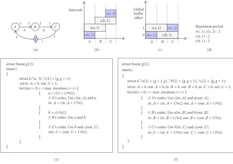
Figure11: (a) A graph which is equivalent toFigure 3a, (b) lifetime intervals of samples for an iteration cycle, (c) an optimal global buffer lifetime chart, (d) repetition periods of sample lifetime patterns, (e) generated code with dynamic binding, and (f) generated code with static binding.
the next iteration cycle as shown in Figure 10b. Then, the period becomes ni=1pi+ 1. Since the sample lifetime
pat-terns over iteration cycles are permutations of each other, sample 1 should be mapped to amongnglobal buffers as-signed to samples 1 throughnduring previous iterations. As illustrated in Figure 10b, other global buffers are occupied
by other samples atk+ni=1pi+ 1 except the global buffer
mapped to tn. Therefore, sample 1 is mapped to the same
global buffer at the next iteration cycle.
We apply the above theorem to the case of Figure 4b
where head interval s(b,3) and tail interval s(b,1) are mapped to the different global buffers. And the sample life-time spans two iteration cycles. Therefore, the repetition pe-riod becomes 2 andFigure 8confirms it.
Another example graph is shown in Figure 11a, which is identical to the simplified H.263 encoder example of
Figure 3. There is a delay symbol on arcCAwith a number inside which indicates that there is an initial samples(c,1). Assume that the execution order isABC. During an itera-tion cycle, samples(c,1) is consumed byAand a new sam-ple s(c,2) is produced byC as shown in Figure 11b. If we expand the lifetime chart over two iteration cycles, we can
notice that head intervals1(c,2) is extended to tail interval
s2(c,1) at the second iteration cycle. By interval scheduling,
an optimal mapping is found likeFigure 11c. ByTheorem 2, the mapping patterns ofs(c,1) ands(c,2) repeat every other iteration cycles since head interval s(c,2) is not mapped to the same global buffer as tail intervals(c,1).
Initial samples also affect the lifetime patterns of sam-ples on the other arcs if they are mapped to the same global buffers as the initial samples. InFigure 11c, samples(b,1) are mapped to the same global buffer withs(c,1) whiles(a,1) with s(c,2). As a result, their lifetime patterns also repeat themselves every other iteration cycles. The summary of rep-etition periods is displayed inFigure 11d.
Recall that the repetition periods determine the period of pointer update in the generated code with dynamic binding strategy, and the size of local buffers in the generated code with static binding strategy. Figures 11e and11fshow the code segments that highlight the difference.
A 1 6 2 B 1 1 C 1 1 D
a b c
(a)
A B C A D
0 1 2 3 4 5 6 7 Global
buffer offset
s(a,3)
s(a,4)
s(a,5)
s(a,6)
s(a,7) (head)
s(c,1)
s(a,1) (tail)
s(a,2) (tail) s(a,8) (head)
s(b,1)
(b)
Repetition period
s(a,1), s(a,3), s(a,5), s(a,7) : 4
s(a,2), s(a,4), s(a,6), s(a,8) : 3
s(b,1) : 1
s(c,1) : 4 (c)
structGg[8]; main() {
structG∗a0[4]={g+ 4, g, g+ 2, g+ 5},∗a1[3]={g+ 6, g+ 1, g+ 3}, ∗b[1]={g+ 7},∗c[1]={0};
for(inti=0;i <max iteration;i++){
{ structG∗output=a0[(i+ 3)%4]; //A’s codes
}{ structG∗input[2];
input[0]=a0[i%4]; input[1]=a1[i%3]; //B’s codes
}{ c[0]=a0[i%4]; //C’s codes
}{ structG∗output=a1[(i+ 2)%3]; //A’s codes
}{
//D’s codes }
} }
(d)
Figure12: (a) An SDF graph with large initial samples, (b) an optimal global buffer lifetime chart, (c) repetition periods of sample lifetime
patterns, and (d) generated code with dynamic binding after dividing local buffers on arcABinto two local buffer arrays.
binding. When the size of a local buffer is the same as the number of newly produced samples within an iteration, no buffer index is needed for the buffer in the generated inlined code. The mapped offset of samples(a,1) repeats every other cycles as that ofs(c,2) does. The mapped offset ofs(b,1) fol-lows that ofs(c,1). For arcCA, the minimum size of local buffers is one since there is at most a live sample on the arc. But we notice that if we have a local buffer on the arc, we need to update the pointer value of each local buffer at every access since the repetition period is two. Therefore, we allo-cate two local buffers on arcCAand fix the buffer pointers. Instead, we update the local buffer indices, in Afor blockA and out Cfor blockC. The decision of the binding scheme is automatically taken care of by the algorithm.
The static binding requires two local pointer buffers for arcABandBC, respectively, since the mapping patterns of samples onAB repeat every other iteration cycles. The
lo-cal buffer size for arcCAis two and has the same binding as
Figure 11e.Figure 11frepresents a generated code with static binding, which additionally requires buffer indices for local buffers on arcABandBC [16]. Hence, we add additional code of updating buffer indices before and after the associ-ated block’s execution. We should consider this overhead to compare the static binding with the dynamic binding strate-gies. In this example, using the dynamic binding strategy is more advantageous.
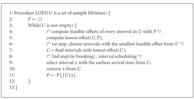
1: Procedure LOES(Uis a set of sample lifetimes){ 2: P← {}
3: While(Uis not empty){
4: /* compute feasible offsets of every interval inUwithP*/ 5: compute lowest offset(U, P);
6: /* 1st step: choose intervals with the smallest feasible offset fromU*/ 7: C←find intervals with lowest offset(U);
8: /* 2nd step(tie breaking) : interval scheduling */ 9: select intervalxwith the earliest arrival time fromC; 10: removexfromU.
11: P←PU{x}.
12: }
13:}
Figure13: Pseudocode of LOES algorithm.
buffer as head intervals(a,7). On the other hand, samples s(a,2),s(a,4),s(a,6), ands(a,8) repeat their lifetime patterns every three iteration cycles since tail intervals(a,2) and head interval s(a,8) are mapped to the same global buffer. The static binding method allocates twelve local buffers to arcAB since the overall repetition period of local buffers on arcAB becomes twelve that is equal to the least common multiple of 4 and 3 (=LCM(4,3)). The dynamic binding method, how-ever, allots two local buffer arrays that have four and three buffers, respectively, to arcAB. Hence the dynamic binding method can reduce five local pointer buffers than the static binding. A code template with inlined coding style is dis-played inFigure 12d. The local buffer pointer for arcCD fol-lows that of samples(a,1).
Up to now, we assume that all samples have the same size. The next two sections will discuss the extension of the pro-posed scheme to a more general case, where samples of dif-ferent sizes share the same global buffer space.
5. BUFFER SHARING FOR DIFFERENT SIZE SAMPLES WITHOUT DELAYS
We are given sample lifetime intervals which are determined from the scheduled execution order of blocks. The optimal assignment problem of local buffer pointers to the global buffers is nothing but to pack the sample lifetime intervals into a single box of global buffer space. Since the horizon-tal position of each interval is fixed, we have to determine the vertical position, which is called the “vertical offset” or simply “offset.” The bottom of the box, or the bottom of the global buffer space has offset 0. The objective function is to minimize the global buffer space. Recall that if all samples have the same size, interval scheduling algorithm gives the optimal result. Unfortunately, however, the optimal assign-ment problem with intervals of different sizes is known to be NP-hard. The lower bound is evident from the sample life-time chart; it is the maximum of the total sample sizes live at any time instance during an iteration. We propose a simple but efficient heuristic algorithm. If the graph has no delays (initial samples), we can repeat the assignment every
itera-tion cycle. Graphs with initial samples will be discussed in the next section.
The proposed heuristic is called LOES (lowest offset and earliest start time first). As the name implies, it assigns inter-vals in the increasing order of offsets, and in the increasing order of start times as a tie breaker. At the first step, the algo-rithm chooses an interval that can be assigned to the small-est offset, among unmapped intervals. If more than one in-terval is selected, then an inin-terval is chosen which starts no later than others. The earliest start time first policy allows the placement algorithm to produce an optimal result when all samples have the same size since the algorithm is equivalent to the interval scheduling algorithm.
The detailed algorithm is depicted inFigure 13. In this pseudocode, U indicates a set of unplaced sample lifetime intervals andP a set of placed intervals. At line 5, we com-pute the feasible offset of each interval inU. SetCcontains intervals whose feasible offsets are lowest among unplaced intervals at line 7. We select the interval with the earliest start time inCat line 9 and place it at its feasible offset to remove it from Uand add it to P. This process repeats until every interval inUis placed.
Since the LOES algorithm can find intervals with lowest offset inO(n) time and choose the earliest interval among them inO(n), wherenis the number of lifetime intervals, it hasO(n) time complexity to assign an interval. Therefore the time complexity of the algorithm isO(n2) fornintervals.
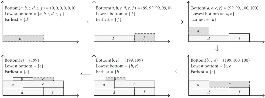
Figure 14 shows an example graph where the circled
number on each arc indicates the sample size. Figure 14b
presents a schedule result and the resultant sample lifetime intervals.Figure 15shows the procedure of the LOES algo-rithm at work. At first, we selectdwith the earliest start time first among the intervals that can be mapped to lowest offset 0. Next, f is selected and placed since it is the only inter-val that can be placed at offset 0. In this example, the LOES algorithm produces an optimal assignment result. With ran-domly generated graphs, it gives near-optimal results most of the time as shown later.
F
100
f E
1
e D
99
d A
100
a B
1
b C
99
c
(a)
F E D C B A
a d b
c e
f
Samples
(b)
Figure14: (a) An input graph with samples of different sizes and (b) a schedule (=ABCDEF) and the resultant sample lifetime chart.
f d
a c
Bottom(b, c, e)=(199,100,100) Lowest bottom={c, e}
Earliest={c}
f d
a c
b
Bottom(b, e)=(199,199) Lowest bottom={b, e}
Earliest={b}
f d
c a
b e
Bottom(e)=(199) Lowest bottom={e}
Earliest={e}
d
Bottom(a, b, c, d, e, f)=(0,0,0,0,0,0) Lowest bottom={a, b, c, d, e, f}
Earliest={d}
d f
Bottom(a, b, c, d, e, f)=(99,99,99,99,0) Lowest bottom={f}
Earliest={f}
d f
a
Bottom(a, b, c, e)=(99,99,100,100) Lowest bottom={a, b}
Earliest={a}
Figure15: The proposed placement algorithm at work.
their heuristic gives similar performance with randomly gen-erated graphs, it does not guarantee to produce optimal re-sults when all samples have the same size.
6. BUFFER SHARING FOR DIFFERENT SAMPLE SIZES WITH INITIAL SAMPLE DELAYS
In this section, we discuss the most general case where a graph has initial samples and samples have different sizes. The LOES algorithm is not directly applicable to this case.
Figure 16 illustrates the difficulty with a simple example.
Figure 16ashows a mapping result after the LOES algorithm is applied to the first iteration period. We assume that “h” and “t” indicate the head interval and the tail interval of the same sample lifetime, respectively. At the second iter-ation, interval h should be placed as shown in Figure 16b
since it is extended from the first cycle. The head inter-val hprohibits interval xfrom lying on contiguous mem-ory space at the second iteration. Such splitting is not al-lowed in the generated code since the code regards each sample as a unit of assignment. To overcome this diffi-culty, we enforce that multicycle intervals do not share the global buffer space with other intervals with different sample size.
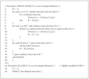
Figure 17displays the main procedure, ASSIGN MAIN,
for the proposed technique. We first classify intervals into several groups (lines 2–13 in Figure 17); a new group is formed with all intervals of the same size if there is at least one multicycle interval, and is denoted as D(x) wherexis the sample size. If there is no multicycle interval, all re-maining intervals form the last groupR. Consider an exam-ple ofFigure 18awhere sample sizes are indicated as circled numbers on the arcs. The sample lifetimes are displayed in
Figure 18b. We make three groups of intervals for this graph. Group D(100) includes all sample intervals associated with arcsb,c, anddwhile groupD(200) includes all intervals as-sociated with arcsaande. Initially groupRis empty in this example.
The next step is to apply the LOES algorithm for each group D(x) since D(x) contains samples of the same size only (lines 14–17). We slightly modify the LOES algorithm so that the algorithm finishes the mapping as soon as all mul-ticycle intervals are mapped: compare line 24 of Figure 17
y t
h x
Global buffer offset
(a)
t y y
t h x
Global buffer offset
1st iteration 2nd iteration Split
(b)
Figure16: (a) A global buffer lifetime chart with different size samples wheretis a tail interval andhis a head interval. (b) Intervalxshould be split at the second iteration, which is not allowed in the generated code.
1: Procedure ASSIGN MAIN(Uis a set of sample lifetimes){ 2: R← {}
3: for eachxinU{/* classify intervals and sort them */ 4: if (xis delayed interval)
5: D(size(x))←D(size(x)){x}
6: else R←R{x}
7: }
8: for eachxinR{/* add ordinary intervals intoD(x) */
9: if(there is a delayed interval whose size is equal to that ofx){ 10: D(size(x))←D(size(x)){x}
11: R←R− {x}
12: }
13: }
14: for eachD(size){/* place intervals inD(x) */ 15: call M LOES (D(size)).
16: R←RD(size) 17: }
18: /* place ordinary intervals inR*/ 19: call LOES(R).
20: } 21:}
22: Procedure M LOES(Uis a set of sample lifetimes){ /* slightly modified LOES */ 23: P← {}
24: While(Uhas delayed intervals){
· · ·
Figure17: Pseudocode of the proposed algorithm for a graph with delays.
into R. Similarly, ordinary interval s(e,2) and s(a,1) are moved into R after s(e,3) is placed for groupD(200). At last we apply the original LOES algorithm to groupR(line 19 of Figure 17) as shown inFigure 18e. The algorithm lo-cates intervals s(c,2), s(e,2), and s(a,1) inR as shown in
Figure 18e.
After all intervals are mapped to the global buffers, we move to the next stage of determining the local buffer sizes, which is already discussed in Section 4. Repetition periods for s(c,1) and s(c,3) become two since tail interval s(c,1) spans two iteration cycles and is not mapped to the same global buffer ass(c,3) is. Repetition periods ofs(e,1),s(e,2), ands(e,3) become all two. A generated code with static bind-ing is displayed inFigure 18f.
7. EXPERIMENT
In this section, we demonstrate the performance of the pro-posed technique with three real-life examples and randomly generated graphs.
E D
C B
A 1
1
1 2 1 1
1 1 1 2
1 2
a b c d
e
200 100 100 100
200
(a)
E D C C B A D Sample lifetime intervals
s(a,1)
s(b,1)
s(b,2)
s(c,1)
s(c,2)
s(c,3)
s(d,1)
s(d,2)
s(e,1)
s(e,2)
s(e,3)
(b) D A B C C D E
Global buffer offset
s(c,1) s(b,2) s(d,2)
s(d,1)
s(b,1) s(c,3)
s(e,1) s(e,3)
s(e,2)
s(c,2)
s(a,1)
0 100 200 300 500 700 800 900
(e)
E D C C B A D Global
buffer offset
s(c,1) s(b,2) s(d,2)
s(d,1)
s(b,1) s(c,3)
s(e,1) s(e,3)
0 100 200 300 500
(d)
E D C C B A D Global
buffer offset
s(c,1) s(b,2) s(d,2)
s(d,1)
s(b,1) s(c,3)
0 100 200 300
(c)
char g[900]; main() {
structG100∗b[4]={g+ 200, g, g, g+ 200},
∗c[4]={g, g+ 700, g+ 200, g+ 700},
∗d[4]={g+ 100, g, g+ 100, g+ 200}; structG200∗a[1]={g+ 700},∗e[2]={g+ 300, g+ 500}; for(inti=0;i <max iteration;i+ +){
{ //D’s codes }{ //A’s codes }{ //B’s codes }{ //C’s codes }{ //C’s codes }{ //D’s codes }{ //E’s codes }
} }
(f)
Figure18: (a) A graph with samples of different sizes and delays, (b) a sample lifetime chart, (c) LOES placement of samples whose size is
Figure19: JPEG encoder example that represents a graph of same size samples without delays.
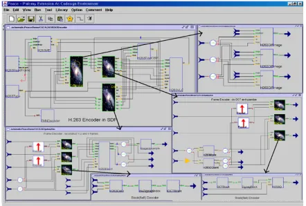
Figure20: H.263 encoder example that represents a graph of dif-ferent size samples with delays.
performance comparison results inTable 1. Since the func-tion body of each dataflow node is equivalent in all experi-ments, only buffer memory requirements are the main item of comparison and the execution times are all similar except for the buffer copy overhead to be discussed below.
A JPEG encoder example represents the first and the sim-plest class of program graphs in which all nonprimitive data samples have the same size and no initial delay exists. Since the local buffer size of each arc is one in this example, we do not have to separate the local pointer buffer and the global data buffer, which is taken into account in the implementa-tion of the proposed technique. We can reduce the memory requirements to one third as the third and the fourth rows of
Table 1illustrate. The last row indicates the lower bound of global buffer requirements that a given execution sequence of nodes needs. The lower bound is nothing but the maxi-mum total size of data samples live at any instance of time during an execution period. No better result is possible since it is optimal.
An MP3 decoder example is composed of three kinds of different size samples. It represents the second class of graphs that have different size samples but no initial delay sample. In this example, we also do not have to separate local and global buffers because the local buffer size of each arc is one. The proposed algorithm that shares the buffer space between dif-ferent size samples reduces the memory requirement by 52% compared with any sharing algorithm that shares the buffer space among only equal size samples. The fourth and the fifth
rows show the performance difference. The proposed algo-rithm also achieves the lower bound in this example.
As for an H.263 encoder example, we make two ver-sions: the simplified version as discussed in the first section and the full version. The simplified version is an example of the third class of graphs in which all nonprimitive data samples have the equal size and initial delay samples exist. As discussed earlier, separation of local buffers from global buffers allows us to reduce the buffer space to optimum as the sixth row reveals. The full version of an H.263 encoder example represents the fourth and the most general class of graphs that consist of different size samples and initial sam-ples. The H.263 encoder example include four different size sample sizes and eight initial delay samples on eight diff er-ent arcs. The proposed technique can reduce the memory re-quirement by 40% compared with the unshared version. On the other hand, a sharing technique reduces the buffer size only 23% if neither buffer separation nor sharing between different samples is considered. In this sample, we cannot achieve the lower bound but 256 bytes larger buffer space. Note that the lower bound is usually not achievable if differ-ent size samples and initial samples are involved in the same graph.
The SDF model has a limitation that it regards a sample of nonprimitive type as a unit of data delivery. In an H.263 encoder example, the SDF model needs an additional block that explicitly divides a frame into 99 macroblocks, paying nonnegligible data copy overhead and extra frame-size buffer space. In a manually written reference code, such data copy is replaced with pointer operation.Table 2reveals this observa-tion: that even the lower bound of memory requirements of the synthesized code from the SDF model is greater than that of the reference code. Therefore, we apply the proposed tech-nique to an extended SDF model, called cyclo-static dataflow (CSDF) [17]. With the CSDF model, we could remove such data copy overhead. And the proposed buffer sharing tech-nique further reduce the memory requirement by 17% more than the reference code.
In the experiments, we choose the better binding strat-egy, static or dynamic, for each data samples, considering the buffer memory and the code overhead of index updates. In the H.263 encoder example, static binding is preferred for places where the repetition periods of sample lifetimes span more than one iteration cycle. In this example, the pointer referencing through local buffers incurs runtime overhead, which is about 0.16% compared with the total execution time in the H.263 encoder.
Table1: Comparison of buffer memory requirements for three real-life examples.
Example JPEG MP3 Simplified H.263 H.263 encoder
encoder
Class Same size Different size Same size Different size
No delay No delay With delay With delay
# of samples 6 336 3 1804
Without buffer sharing 1536 B 36 KB 111 KB 659 KB
Sharing buffers of same size only 512 B 23 KB 111 KB 510 KB
Buffer sharing without buffer separation 512 B 11 KB 111 KB 510 KB
Buffer sharing with buffer separation — — 74 KB 396 KB
Lower bound of global buffer size 512 B 11 KB 74 KB 396 KB
Table2: Comparison of synthesize codes with reference code for the H.263 encoder.
Example Reference code Buffer sharing without Buffer sharing with
buffer separation in CSDF buffer separation in CSDF
H.263 Encoder 350 KB 291 KB 290 KB
Table3: Performance comparison of LOES algorithm with integer linear programming (optimal) for randomly generated graphs (unit: %).
# of intervals 5 7 9 11 13 15 20 Avg. max
(LOES-ILP)/ILP 0.0 0.0 0.1 0.1 0.5 0.3 0.3 0.2 14
8. CONCLUSIONS
We have proposed a buffer sharing technique for data sam-ples of nonprimitive type to minimize the buffer memory requirements from graphical dataflow programs based on the SDF model or its extension assuming that the execu-tion order of nodes is already determined at compile time. In order to share more buffers, the proposed technique sep-arates global memory buffers from local pointer buffers: the global buffers store live samples and the local buffers store the pointers to the global buffer entries. The technique min-imizes the buffer memory by sharing global buffers for data samples of different size. No previous work is known to us to solve this sharing problem especially for the graphs with initial samples. It also involves three subproblems of map-ping local pointer buffers onto the global buffer space, deter-mining the local buffer sizes, and finding the repeating map-ping patterns.
We first obtain the minimum size of global buffer spaces assuming that local pointer buffers take negligible amount of buffer space compared with the global buffer space. A LOES algorithm has been developed for buffer sharing be-tween samples of different sizes. The next step was to bind the local pointer buffers to the given global buffers for the graph. We present both dynamic binding and static binding meth-ods and compare them in terms of memory requirements and code overheads. The proposed technique, including
au-tomatic code generation and memory optimization, has been implemented in a block diagram design environment called PeaCE. No manual intervention is necessary for the proposed code generation technique in PeaCE.
The experimental results show that the proposed algo-rithm is useful, especially for the graphs with initial de-lays. The proposed algorithm that separates local buffers and global buffers reduce more memory by 33% in the simplified H.263 encoder and 22% in the H.263 encoder than the shar-ing algorithm that does not separate local buffers and global buffers. Through extensive buffer sharing optimizations, au-tomatic software synthesis from a dataflow program graph achieves the comparable code quality with the manually op-timized code in terms of memory requirement.
In this paper, we assume that the execution order of blocks is given from the compile-time scheduling. In the fu-ture, we will develop an efficient scheduling algorithm which minimizes the memory requirement based on the proposed algorithm.
ACKNOWLEDGMENTS
REFERENCES
[1] COSSAP User’s Manual, Synopsys, Mountain View, Calif, USA.
[2] R. Lauwereins, M. Engels, J. A. Peperstraete, E. Steegmans, and J. Van Ginderdeuren, “GRAPE: a CASE tool for digital signal parallel processing,”IEEE ASSP Magazine, vol. 7, no. 2, pp. 32–43, 1990.
[3] J. T. Buck, S. Ha, E. A. Lee, and D. G. Messerschmitt, “Ptolemy: a framework for simulating and prototyping het-erogeneous systems,” International Journal of Computer Sim-ulations, vol. 4, no. 2, pp. 155–182, 1994.
[4] E. A. Lee and D. G. Messerschmitt, “Static scheduling of synchronous dataflow programs for digital signal processing,”
IEEE Trans. on Computers, vol. 36, no. 1, pp. 24–35, 1987. [5] Telenor Research, “TMN (H.263) Encoder/Decoder Version
2.0,” June 1997,ftp://bonde.nta.no/.
[6] P. K. Murthy, S. S. Bhattacharyya, and E. A. Lee, “Joint min-imization of code and data for synchronous dataflow pro-grams,” Journal of Formal Methods in System Design, vol. 11, no. 1, pp. 41–70, 1997.
[7] W. Sung, J. Kim, and S. Ha, “Memory efficient software syn-thesis from dataflow graph,” in11th International Symposium on System Synthesis (ISSS ’98), pp. 137–144, Hsinchu, Taiwan, December 1998.
[8] S. S. Bhattacharyya, P. K. Murthy, and E. A. Lee, “APGAN and RPMC: Complementary heuristics for translating DSP block diagrams into efficient software implementations,”Journal of Design Automation for Embedded Systems, vol. 2, no. 1, pp. 33– 60, 1997.
[9] F. J. Kurdahi and A. C. Parker, “REAL: a program for register allocation,” inProc. 24th ACM/IEEE Design Automation Con-ference (DAC ’87), pp. 210–215, Miami Beach, Fla, USA, June 1987.
[10] M. R. Garey, D. S. Johnson, and L. J. Stockmeyer, “Some sim-plified NP-complete graph problems,” Theoretical Computer Science, vol. 1, no. 3, pp. 237–267, 1976.
[11] J. Gergov, “Algorithms for compile-time memory optimiza-tion,” inProc. 10th Annual ACM-SIAM Symposium on Discrete Algorithms (SODA ’99), pp. 907–908, Baltimore, Md, USA, January 1999.
[12] E. De Greef, F. Catthoor, and H. D. Man, “Array placement for storage size reduction in embedded multimedia systems,” inProc. International Conference on Application-Specific Array Processors (ASAP), pp. 66–75, Zurich, Switzerland, July 1997. [13] P. K. Murthy and S. S. Bhattacharyya, “Shared buffer
imple-mentations of signal processing systems using lifetime analy-sis techniques,”IEEE Transactions on Computer-Aided Design of Integrated Circuits and Systems, vol. 20, no. 2, pp. 177–198, 2001.
[14] S. Ritz, M. Willems, and H. Meyr, “Scheduling for optimum data memory compaction in block diagram oriented software synthesis,” inProc. IEEE Int. Conf. Acoustics, Speech, Signal Processing, pp. 2651–2653, Detroit, Mich, USA, May 1995. [15] F. Gavril, “Algorithms for minimum coloring, maximum
clique, minimum covering by cliques, and maximum inde-pendent set of a chordal graph,”SIAM Journal on Computing, vol. 1, no. 2, pp. 180–187, 1972.
[16] S. S. Bhattacharyya and E. A. Lee, “Memory management for dataflow programming of multirate signal processing al-gorithms,” IEEE Trans. Signal Processing, vol. 42, no. 5, pp. 1190–1201, 1994.
[17] G. Bilsen, M. Engels, R. Lauwereins, and J. A. Peperstraete, “Cyclo-static data flow,”IEEE Trans. Signal Processing, vol. 44, no. 2, pp. 397–408, 1996.
Hyunok Oh is a Ph.D. candidate in the School of Computer Science and Engineer-ing at Seoul National University, Korea. He received his B.A. degree (1996) and M.A. degree (1998) in computer engineer-ing from Seoul National University, and he is in a Ph.D. program from 1998 to 2002. He is interested in hardware-software codesign, model of computation, hardware-software cosynthesis, memory optimiza-tion, and multimedia applications.
Soonhoi Hais currently an Associate Pro-fessor in the School of Electrical Engineer-ing and Computer Science at Seoul National University. From 1993 to 1994, he worked for Hyundai Electronics Industries Corpo-ration. He received his B.A. degree (1985) and M.A. degree (1987) in electronics en-gineering from Seoul National University, and Ph.D. (1992) degree in electrical engi-neering and computer science from