R E S E A R C H
Open Access
Source positioning in a large-scale tiny-sensor
network of arbitrary topology
Dmitriy Penkin
1*, Gerard Janssen
2and Alexander Yarovoy
1Abstract
To effectively localise a source node in a dense wireless tiny-sensor network with an arbitrary 2D/3D node distribution, a novel approach suitable to describe the hop progress of source-to-sink path in such a system is proposed. In this approach, the network topology is described as a regular lattice and relates the statistical parameters of the hop count in the source-to-sink propagation path to the fractal properties of a percolating cluster. Based on this approach, a mathematical model is developed to estimate the probabilityP(r,t)of successful reception of the message by a sink node spaced at distancerfrom a source in a given timet. The accuracy analysis of the positioning method
demonstrates its high performance for the very broad spectrum of values of the occupation probabilitypocc.
Keywords: Random network; Lattice model; Percolation theory; Multihop channel; Hop count; Source-to-sink path; Localization algorithm
1 Introduction
At present, environmental sensing using electromagnetic waves can be performed using two different approaches. The first approach implies the use of devices that sense an environment remotely (e.g. radars or lidars). Another approach requires a number of sensor nodes, which are distributed in an application area, perform sensing directly inside the phenomenon and wirelessly commu-nicate with each other and with the external reference nodes (sinks). The collected local data are then transmit-ted through such a wireless sensor network towards an end user in a multihop fashion. The ability to operate and monitor in harsh, complex and inaccessible environ-ments makes the latter approach more promising and ensures a wide range of applications for wireless sen-sor networks. In particular, there already exist low-end sensor-network-based solutions aiming to detect a sniper location [1], monitor volcano intensity [2], protect for-est against fire [3], control water waste in homes [4] and the like [5]. All these actual sensor networks consist of a small number of macro-scale nodes with their posi-tions carefully engineered or pre-determined and capable of coarse-grained sensing. Further development of such
*Correspondence: [email protected]
1Microwave Sensing, Signals and Systems Group, Delft University of Technology, Mekelweg 4, Delft 2628CD, The Netherlands Full list of author information is available at the end of the article
sensor networks towards a wireless tiny-sensor network (WTSN) with superior fine-grained sensing capabilities would enable a wide spectrum of appealing applications in civil engineering and the health-care sector [6]. Simi-lar to its macro-scale counterpart, each node in a WTSN integrates a sensing, processing and communication unit and a power source [7]. Due to its size restrictions, the tiny node imposes severe constraints on its power component [8]. Since the communication coverage of such a node is thus very limited, the WTSN is foreseen as a swarm of densely deployed nodes within an application area: due to the high node density, the network can still support a long-distance transmission using multihop communica-tion. The simple functionality of tiny nodes implies that the WTSN topology cannot be retrieved (a node has no energy to reconnoitre its surroundings). A large number of these nodes in turn entails that a random scattering over the area to be monitored is the most convenient or perhaps the only option to deploy them. All these features make the WTSN very distinguishable from the current sensor systems. Therefore, novel solutions at the network-ing level are needed to transfer and extract information gathered by the WTSN.
In particular, an efficient method capable of localising a transmitting node in the WTSN is required. The use of GPS on all nodes is unacceptable in terms of energy resources, node dimensions and its inability to operate
indoor, so other techniques have to be considered. At present, there are two such major GPS-free techniques for positioning in multihop environments: centralised and distributed localisation. In the first approach, all ranges between all nodes in the network are measured, marked by unique node numbers and are transmitted to a global central unit, which processes and computes the location of each node in the network [9-11]. Evidently, the cen-tralised approach is not a good candidate for the WTSN since it requires a very large communication overhead. Distributed localisation algorithms [12-15] require com-munication and ranging only with direct neighbouring nodes and are in general more robust and energy effi-cient than centralised schemes. With distributed localisa-tion, each node in the network is capable of processing and computing to remove a lack of reliance on a sin-gle point of possible failure and provide with an opti-mum load balancing. Both approaches mentioned above require a large amount of energy to perform the prereq-uisite self-organization stage since the nodes must recon-noitre their surroundings to form a network topology. Due to modest processing capabilities and very limited energy resources of the nodes, the distributed localisa-tion however becomes unaffordable and impracticable for the WTSN. In view of this, we propose a pioneer-ing approach to estimate the location of a source node in the WTSN with arbitrary positions of nodes without con-suming extra energy on the self-organization step. This approach employs an analysis of hop progress in such a network and uses time differences of last-arriving signals to its borders to position a source (initially transmitting) node.
Due to the complexity and the unknown locations of sensor nodes, determination of the hop count in the source-to-sink path of the WTSN is intractable with exist-ing solutions, which are based on statistical laws (e.g. the Poisson distribution). Models available in the literature on the probabilistic analysis of the hop count in a large-scale and decentralised system are currently limited to two-dimensional (2D) networks. In particular, the probability of establishing a connection of a given length through a planar network with uniformly distributed nodes with a given number of hops has been investigated in [16]. There it was shown that node density does not greatly affect the hop count but has a huge effect on whether a connection can be made at all. In turn, the distribution of Euclidean distances to thenth node in a Poisson process is studied in [17]. For homogeneous sensor networks, the connec-tivity probability in one or two hops is derived and the connectivity in multiple hops is examined with analyti-cal bounds in [18]. In [19], the distribution of the hop distance and its expected value in uniformly distributed networks are analysed by means of numerical simula-tions. The results indicate that directional nodes might
substantially decrease the hop count compared to omni-directional ones, although the connectivity of a large-scale sensor system will degrade. Hence, as there are merely solutions suitable to determine the hop count in specific 2D WTSN structure, which require heavy computational resources to treat large-scale networks, a different model capable of analysing the source-to-sink multihop path in a 2D/3D WTSN and obtaining its hop count in a low-cost manner is developed here. It is notable that the model capable of analysing the hop progress can also be used to estimate the time required to pass a message through the WTSN and reach a sink node as well as determine other relevant parameters, such as degradation of network throughput and raised source localization cost [20-22].
In the proposed model, the WTSN topology is mapped to a regular lattice, where each lattice site is occupied by a sensor node with certain occupation probability. By relating statistical parameters (such as mean and vari-ance) of the source-to-sink hop count to fractal properties of the percolating cluster in the corresponding lattice, the probability P(r,t) of successful reception of sensed data by a sink node spaced at Euclidean distancerfrom a source in a given time interval t can in particular be estimated. This probability quantifies the source-to-sink channel in the WTSN and may be regarded as a mea-sure of the network reliability. Based on the hop progress model, the new positioning algorithm that requires no energy on the self-organization step is eventually proposed.
The remainder of the paper is organized as follows. Concepts of percolation theory and the system mod-elling from the percolation perspective are discussed in Section 2. In Section 3, a technique to determine the hop count of the source-to-sink channel in a WTSN and the probability P(r,t) is developed, whereas simulation and numerical results are provided in Section 4. Finally, the source-positioning method for the WTSN is introduced and discussed in Section 5, whereas the paper concludes in Section 6.
2 System model
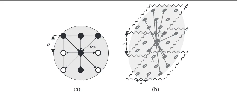
In this paper, the 2D area of interest is discretized in a regular square lattice with a2 = b2/
√
2, and thus, the amount of sites to be reached through an one-hop link (i.e. adjacent) is limited by the node degree number
m2 = 8 (Figure 1a). In turn, the 3D application space is simplified to a regular cubic lattice witha3 = b3/
√
3, and consequently, the number of adjacent sites is lim-ited tom3 = 26 (Figure 1b). Both selected structures are chosen so to be conceptual since any square/cubic lat-tice with latlat-tice spacinga2 < b2/
√
2 (a3 < b3/
√
3) can be converted to such a corresponding structure using the position-space renormalization group technique and be subsequently resolved [24].
Due to the regularity, the probability that a site of this lattice is occupied by a node is uniform and can be obtained aspocc=ρ·(ad)d, whereρis the given node den-sitym−d, and (a
d)d indicates thed-dimensional space occupied by a single site. Two occupied sites are inter-connected only if either there exists a one-hop link or both of them share such links with another occupied site. The one-hop link exists solely when the sites are spaced at a distance less thanbd, while occupied sites separated by a large range (i.e. bd) can still establish a connec-tion through a multihop channel. The occupied sites form clusters in the lattice. When the occupation probability
poccis small, there is a sparse population of occupied sites, and clusters composed of small numbers of these sites predominate. However, by increasingpocc, more occupied sites become interconnected and thus become part of the same cluster. Eventually, forpoccto be large enough, the lattice experiences a critical phase transition: i.e., once
pocc reaches the percolation threshold pc, an infinitely large percolating cluster of interconnected sensor sites emerges for the first time [25]. For a finite-sized lattice,
this cluster is bounded by the lattice edges, thus also called the spanning cluster [26]. The percolation threshold value
pcdepends merely on the lattice geometry and the ‘lattice’ node coverage: the number and organization of sites are interconnected through a one-hop link. Note that due to an exceedingly complex structure of the percolating clus-ter in higher dimensions, it is cumbersome to declus-termine the percolation threshold analytically except for the 1D and a few 2D lattices [27]. In this respect, the valuepcis typically estimated via a numerical experiment.
Whenpocc < pc, the WTSN is basically fragmented, i.e. composed of many disjoint clusters. Therefore, due to the finite size of a cluster, in which the source node is located, the probability to receive sensed data abruptly goes to zero with increasing source-to-sink separation. In this way, such a sensor network is unreliable and its mod-elling will not be treated in this paper. Oncepocc>pc, the WTSN becomes a dependable system since at any source-to-sink distance, there always exists a multihop channel between two arbitrary chosen occupied sites when they belong to the percolating cluster. Hence, the probability
P(r,t)that a node at Euclidean distancerfrom a source receives a message in a time intervaltcan be decomposed as
P(r,t)=p(r,t)·p2cl, (1) where pcl is the probability a site belongs to the perco-lating cluster (the power of two is due to the fact that both source and sink nodes must be part of this clus-ter), whereasp(r,t) is the probability a signal conveyed through such a cluster is received within the time inter-valtby the sink node at the distancerfrom the source. The analysis ofpclis carried out in Section 4, while the probabilityp(r,t)is modelled in the next section.
(a)
a
(b)
b
(2)a
b
(3)a
3 Signal flooding modelling
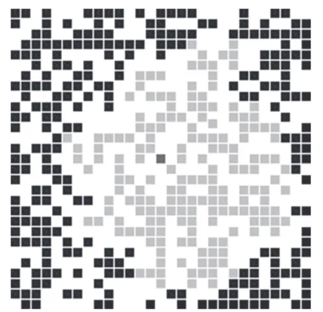
The probabilityp(r,t)is determined based on the diffu-sion process defined on the sites of a percolating cluster. In particular, the time variable t is considered discrete. Note that the time unit is determined by the processing delay time in a sensor nodetas it is much larger in gen-eral than the propagation time. In other words, at each time unitt, a message is regarded to hop from its cur-rent positions to adjacent occupied sites, i.e. the signal propagates in a flooding manner. Hence, in time intervalt, the sensed signal propagating in a wavefront manner per-formsh= t/thops and the occupied nodes, which are eventually reached, form an aggregation. For the sake of understanding, such a particular aggregation forh=20 in the 2D lattice of interest withpocc =0.5 is demonstrated in Figure 2.
Since any aggregation is obviously inscribed by a circle (or a sphere for 3D) with its centre coincided with a source site and radius ofh·b, the probabilityp(r,t)is a non-zero value only when the number of hopshin time intervalt
exceeds the minimum hop countn = r/brequired to cover a distancer. To reach a sink node spaced atrin the minimum number of hopsh = nwith probability 1, it is required to have no empty sites in a lattice (i.e.pocc = 1) in order to transmit a signal between sites which are merely located along the source-to-sink direction; thus, the resulting multihop path is a straight line and its frac-tal degree is equal to 1. For a lattice withpocc < 1, the
Figure 2Aggregation of the occupied nodes forh=20 in the 2D lattice characterised bypocc=0.5.The blank sites are drawn in
white; the occupied sites are shown in black. The sites, which belong to the aggregation, are depicted in light grey, while the origin node is displayed in dark grey.
presence of blank sites implies that the fractal degree of the source-to-sink multihop path exceeds 1, and as a con-sequence,h> nhops are needed to cover the distancer. Evidently, in the worst case scenario, the probabilityp(r,t) has to be related to the multihop path with the highest fractal degree, which demands the largest number of hops
hfor reaching the sink at distancer. Since such a ‘longest’ path is composed of the sites situated on the hull of a percolating cluster, statistical parameters of the source-to-sink path can directly be associated with the fractal properties of this cluster hull. As shown in [28,29] and verified in Section 4, the hop count of a path through a cluster hull is typically distributed according to the Gaussian law. Therefore, the multihop path of interest can be defined in terms of its mean and variance, and the probability p(r,t), which is regarded as the cumulative distribution function of its hop count, is expressed as
p(r,t)= 1
whereμandσ are the mean and variance corresponding to the hop count in the ‘hull’ multihop path, respectively. The parameterh is the actual number of hops made in time t, while the minimum number of hops needed to cover the source-to-sink distanceris equal ton. Hence, the probabilityp(r,t)increases monotonically from zero (h < n) to 1 (h μ), whereμformally corresponds to the average number of hops to be made to reach the sink node through a ‘hull’ multihop path.
Since the hull of a percolating cluster does possess frac-tal properties [29], fracfrac-tal principles demand that the parameters μandσ, which describe the multihop path composed of sites appertaining to the cluster hull, are expressed via n as follows (this conclusion is also sup-ported through calculations in [30]):
μ=cμ·ndμ, σ =cσ ·ndσ,
(3)
where c and d are, respectively, the effective amplitude and the fractal (or Hausdorff ) dimension of the Gaussian parametersμandσ. Hence, Equation 2 forp(r,t)can be rewritten using Equation 3 as
p(r,t)= 1 can be determined once the effective amplitudes cμ,cσ
and the fractal dimensionsdμ,dσ are known. Such
are estimated by means of numerical experiments (the modelling is simple and shown in Section 4). It is also notable that once these parameters are known, the prob-abilityp(r,t) can be assessed for any distancerwithout extra numerical simulations as the fractal parameters are independent of the source-to-sink separation. This is an essential advantage of the proposed model since; unlike other simulation solutions, it can treat a very large-scale sensor network in a simple way.
4 Numerical analysis
The percolation thresholdpcand the size of a percolating cluster are numerically explored as both coefficients are of particular interest: the valuepcdistinguishes percolating from fragmented systems, while its size is directly related to the probabilitypclthat an occupied site belongs to the percolating cluster. To determine the fractal parameters related to the cluster hull, the hop count of a multi-hop path only composed of sites belonging to the hull is investigated as well.
To estimate these parameters, a set of Monte Carlo sim-ulations are carried out. Due to computer limitations, the largest source-to-sink distance of a 2D lattice being anal-ysed is 2,000 sites, whereas that of a 3D system is bounded by 500 sites. To get accurate results, each set of numerical experiments requiresQ = 3, 000 iterations. Per simula-tion, a signal is only transmitted to the adjacent occupied sites, which are found based on the left-hand maze rule in order to keep its propagation along the cluster hull (by keeping the left hand in contact with one wall of a maze, the player is guaranteed not to get lost and will reach a different exit if there is one). Once there exists a multihop path between the source site and sink spaced at distance
n, the outcome is assumed to be successful and the hop count h of this path is stored. After applying this pro-cedure Qtimes, the value pc is determined as the ratio between the number of successful outcomes and the total number of iterations, while the mean valueμand the stan-dard deviationσare eventually determined through using their common representations.
The percolation threshold of a 2D structure is found to be equal to pc(2) = 0.4073 ± 0.0007. This result is in
agreement with the data presented in [31]. The percola-tion threshold of a 3D lattice is significantly less thanpc(2)
and determined to bepc(3) = 0.0977 ± 0.0008. The
fur-ther estimations are performed under the assumption that the occupation probability pocc exceeds the percolation threshold to ensure that a percolating cluster arises.
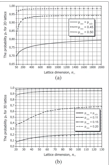
The probabilitypclthat a site belongs to the percolat-ing cluster directly corresponds to the ratio of the number of sites in this cluster and the total number of occu-pied sites. The size of a percolating cluster is determined from numerical simulations on a square and cubic lat-tice, whereas the amount of occupied sites is consequently
expressed aspocc·nd, wheredis the lattice dimension. To understand the behaviour of the probabilitypcl, the size of a percolating cluster is in particular analysed for differ-ent values ofpoccand lattice dimensions. For a 2D and 3D structure, the probability that the starting node belongs to the percolating cluster is found to be reasonably less than 1 in the vicinity of the percolation thresholdpc(Figure 3). Nonetheless, for both lattices of interest, the value ofpcl rapidly tends to 1 once the occupation probability pocc increases. In other words, with raisingpocc, the level of disjoint clustering in a lattice considerably decreases as more and more occupied sites become part of the perco-lating cluster. Hence, althoughpclnever strictly equals 1 as long as some randomness occurs in a WTSN (pocc < 1), for practical applications, the probabilitypclcan be sup-posed to be about 1 since a node density would be chosen such thatpocc is reasonably larger than the respectivepc for ensuring network connectivity. Note that we however rely on the actual values ofpclto obtain accurate results here.
(a)
(b)
For any lattice, the fractal dimensions dμ and dσ are
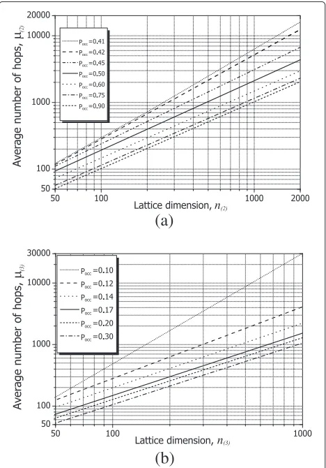
found to reach their maxima when the probabilitypoccis near the percolation thresholdpcand become minimum whenpocctends to 1. The reason for such a behaviour is that by increasing the probability pocc, we decrease the degree of randomness in a network, and consequently, the mean number of hopsμmoves to nas well as the value of σ decreases to zero. To demonstrate that the fractal dimension is the prime characteristic which affects the rate of increase ofμandσ with increasing the value n, the fractal parameters for both 2D and 3D lattices are obtained by fitting the mean and variance of the hop count
hcalculated for different nto Equation 3. These results are shown in Figure 4 (only forμ), whereas the estimated parameters are indicated in Table 1. Also note that such a fractal behaviour is not seen for small hop distancesn
since the percolation theory requires a great number of entities to become applicable. In particular, according to the numerical experiments, it is suggested to keepnlarger than 50 to be able to use this approach.
(a)
(b)
Figure 4Dependence of average hop countμon lattice dimension for (a) 2D and (b) 3D structures.
Table 1 Fractal characteristics of 2D and 3D lattice structures
Fractal parameters Values
pocc(2) 0.41 0.42 0.45 0.50 0.60 0.90
cμ(2) 0.5736 0.8393 1.4337 1.5947 1.4389 1.0169 dμ(2) 1.3469 1.2631 1.1116 1.0410 1.0041 1.0007 cσ (2) 0.1252 0.2560 1.1821 1.9558 1.6301 0.2291 dσ (2) 1.3921 1.2470 0.8479 0.6343 0.5178 0.5022
pocc(3) 0.10 0.12 0.14 0.17 0.20 0.30
cμ(3) 0.1245 1.3137 1.5666 1.4140 1.2569 1.0556 dμ(3) 1.7956 1.1650 1.0508 1.0116 1.0041 1.0004 cσ (3) 0.0153 1.7925 2.7176 1.9873 1.1938 0.3684 dσ (3) 2.0603 0.8296 0.5788 0.5038 0.5033 0.5025
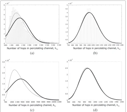
The Kolmogorov-Smirnov criterion is applied to test the suitability of the Gaussian distribution to the random dis-tributions of the hop countsh2andh3for the 2D and 3D systems, respectively. For the sake of curiosity, other major statistical hypotheses are considered as well. In particular, the lognormal distribution fits best both the random dis-tributions of the hop counts. Meanwhile, it has been found that the normal distribution fits well to the calculated random data sets and can fairly describe the arbitrary behaviour of the hop countsh2andh3only ifpoccis more than 0.5 and 0.14, respectively (Figure 5). Nonetheless, the assumption of normally distributed parameterp(r,t) in Equation 4 is valid, and thus, the model still furnishes proper results for the very broad spectrum ofpocc.
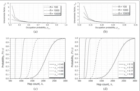
To better understand the actual impact of randomness on the WTSN, a ‘tortuosity’ level of the multihop path along the hull of the percolating cluster is introduced as = μ/nand analysed as a function of the probability
pocc and the hop distancen (Figure 6). As can be seen, the larger the distancenand the smaller the probability
(a)
(b)
(c)
(d)
Figure 5The random distribution histograms are plotted for the 2D lattice of dimensionn(2)=500 with(a)pocc(2)= 0.42 and(b) pocc(2)= 0.50.For the 3D lattice, the dimensionn(3)=300 and the occupation probabilities(c)pocc(3)=0.10 and(d)pocc(3)=0.14. A Gaussian
distribution approximation is depicted in bold, whereas a line following a lognormal distribution is of standard thickness.
ofpoccconsiderably affects such a probability: in partic-ular, the value of P(r,t) increases pretty fast by slightly increasingpocc. From this point, it follows that to meet a common criterion of WTSN-based applications, i.e. to receive a signal with a high probability, it is better to add extra sensors and increase the valuepoccrather than expand the time interval t. Another fact to be empha-sised is that the dimensionality significantly affects the characteristics of a percolating cluster, e.g.dμ(3)decreases
much faster thandμ(2)with increasing occupational
prob-ability due to having an extra degree of freedom in 3D networks. Note also that the Gaussian distribution of the multihop path, which is derived from the results of Monte
Carlo simulations, is depicted in markers in Figure 6c,d and corresponds to pocc(2) = 0.45 and pocc(3) = 0.12,
respectively.
(a)
(b)
(c)
(d)
Figure 6The tortuosity parameterand the probabilityP(r,t)for 2D(a, c)and 3D(b, d)lattices.For panels(c)and(d), the source-to-sink separation isn=700.
the proposed model is relevant for handling such a sys-tem. The source-to-sink path with the maximum num-ber of hops, which can be rigorously defined through the fractal characteristics of the hull of the percolating cluster, is also important from a communication per-spective as its modelling helps to avoid inter-message interference in the WTSN (i.e. the source node must send more than one message to complete its report). How-ever, the proposed model is not limited to such predic-tions on communication properties of a WTSN but also can be used to effectively position a source node in this network.
5 Source-positioning method
Once a source node in the WTSN triggers, its posi-tion is assumed to be detectable only when this node is located at one of the network borders (i.e. an end user can only get access and treat such ‘outward’ sensor nodes). If a message originates from one of the ‘inward’ nodes, there is no direct way to localise this node as it is inaccessible from an end user point of view. Nonethe-less, if such an ‘inward’ source belongs to the percolating cluster, the originating message spreads throughout the
WTSN and is only terminated by the lattice borders. By using the data collected at these borders and apply-ing the developed model of hop progress in the WTSN, the position of the inward source node can reliably be estimated.
The positioning algorithm is, in particular, described for the 3D WTSN. For the sake of simplicity, it is assumed that this area can be represented by a regular lattice of
Ni×Nj×Nk. Once the inward source node with coor-dinates (i,j,k) belongs to the percolating cluster, a sig-nal originating from it and spreading within this cluster reaches all the lattice borders after all (Figure 7). Here-inafter, let us focus on the determination of parameter
Figure 7‘Hull’ multihop paths to the left and right (opposite) borders in a 3D WTSN.The network is simplified by a lattice of dimensionNi×Nj×Nk, and a source node is situated in(i,j,k)site.
and the standard deviation σ (ti) can be expressed as follows:
μ(ti)= μ(tl)−μ(tr)=t[μ(hl)−μ(hr)]=
=t·cμ(3)
idμ(3)−(N
i−i)dμ(3) ;
(5)
σ (ti)=
σ (tl)2+σ (tr)2=
=t·cσ (3)
i2dσ (3)+(Ni−i)2dσ (3),
(6)
where effective amplitudescμ(3) andcσ (3)and the fractal
dimensionsdμ(3) anddσ (3) are obtained as described in
Section 4. In this context, the coordinateiof the source node can be calculated by measuring the delay timestland tr and solving Equation 5 with μ(ti) = tl−tr. Other coordinatesjandkcan be determined in the similar fash-ion by assessing the delay timestjandtk between the respective lattice boundaries.
From Equation 6, by taking ∂{σ (ti)}/∂i = 0, it fol-lows that the maximum standard deviation in sites for the relative timetiis given as follows (this derivation is thoroughly discussed in [30]):
σmax(ti)=
cσ (3)·Nidσ (3)
cμ(3)·N dμ(3)
i
·Ni. (7)
The maximum standard deviation for tj and tk is obtained using the same equation but substituting Ni withNjandNk, respectively. In this regard, the accuracy of the proposed positioning method can be numerically tested by comparing a confidence region of signal ori-gin to the entire lattice area. The confidence region is estimated by using the maximum standard deviation of each of three parameters ti, tj, tk and the normal
distribution quantile function (as all these parameters have the Gaussian distribution) and described as
CR(3)=Z3p·
cσ (3)·N dσ (3)
i
cμ(3)·N dμ(3)
i
·cσ (3)·N
dσ (3)
j
cμ(3)·N dμ(3)
j
×
× cσ (3)·N
dσ (3)
k
cμ(3)·N dμ(3)
k
·Ni·Nj·Nk,
(8)
whereZpis the normal distribution quantile for a known confidence levelp. Since the total number of sites in the lattice isNi·Nj·Nk, the ratio between the confidence region
(a)
(b)
Figure 8Accuracy of source localization (the ratio between the confidence area and the entire lattice area).This characteristic is shown as a function of the lattice dimensionn(2)and the confidence
and the entire lattice area is simplified from Equation 8 as
Evidently, the accuracy of the positioning method for the 2D WTSN can be treated in the same way as above. The ratio(2) is thus reduced from Equation 9 and has
the squaredZpand no term containingNkdue to the two dimensionality.
The analysis of results suggests that the proposed posi-tioning method technique is limited to the cases when the fractal dimensiondσ (2,3) is smaller than the value of
dμ(2,3). Otherwise, the algorithm becomes inaccurate and
unstable as the value of(2,3)would diverge with
increas-ing the lattice sizes. This requirement puts a limit on the occupation probability, such as according to Table 1 for the lattices of interestpocc(2) > 0.42 andpocc(3) > 0.11.
Note that due to the fast decrease ofdσ (2)with increasing
occupational probability, the algorithm accuracy notice-ably improves oncepocc(2) is moderately larger than the
percolation threshold (see Figure 8). For 3D WTSNs, this accuracy refinement is even more substantial due to an extra dimensionality.
6 Conclusions
In this paper, we propose a novel method to obtain in a simple manner the worst case number of hops of the source-to-sink path in a very large-scale network with an arbitrary network complexity and the unknown locations of the wirelessly connected nodes. The model assumes that the network topology can be represented by a regular lattice, where each lattice site is occupied by a sensor node with occupation probability pocc. The value pocc should exceed the percolation thresholdpcfor the emergence of a percolating cluster. Then, by relating statistical parame-ters (such as mean and variance) of the hop count of the source-to-sink path to the fractal parameters of the perco-lating cluster, the probabilityP(r,t)indicating a successful arrival of the sensed signal to a sink node spaced at dis-tancerfrom a source within a specified timethas been mathematically expressed. The simple approach to esti-mate fractal parameters of the percolating cluster based on the left-hand maze rule has been used.
The numerical analysis has been performed for 2D and 3D conceptual lattices to better understand the impact of randomness on a large-scale network. It has been shown that the network withpocc being close topcis an unreli-able system from an application perspective. Meanwhile, it has also been demonstrated that the occupational prob-ability pocc greatly affects the level of randomness in the network, i.e. the valueP(r,t)increases pretty fast by slightly increasingpoccbeyondpc. From this, the practical
conclusion can be drawn that it is more effective to increaseP(r,t)through adding extra sensors rather than by expanding the timet. The raise ofP(r,t)with increas-ing number of sensors is much faster in 3D network than that in 2D due to having an extra degree of freedom. The inverse problem, i.e. the determination of the occupa-tional probability needed to maintain the requiredP(r,t), can also be solved using the developed model. Note that although the model’s applicability is currently limited by nodes radiating omnidirectionally, the approach shown in the paper implies that the model can be expanded to nodes with directional coverage once the fractal parame-ters in the respective lattice structure are estimated.
An effective source-positioning method, which can localise a source node in a large-scale network with arbi-trary positions of nodes and without retrieving the net-work topology, has been proposed based on the developed connectivity model. This localization method, which can be applied in very large scale networks, exploits the frac-tal nature of the percolating cluster. The accuracy analysis of the method has demonstrated its high performance for the very broad spectrum of values of the occupation prob-abilitypocc. As the counterpart approaches are impartially restricted to position in very large-scale networks, this method is the first of its kind to localise a source in these networks and thus is useful for designing such networks in the near future.
Competing interests
The authors declare that they have no competing interests.
Acknowledgements
The authors thank the anonymous reviewers for their constructive and helpful comments.
Author details
1Microwave Sensing, Signals and Systems Group, Delft University of Technology, Mekelweg 4, Delft 2628CD, The Netherlands.2Circuits and Systems Group, Delft University of Technology, Mekelweg 4, Delft 2628CD, The Netherlands.
Received: 21 June 2013 Accepted: 9 April 2014 Published: 28 April 2014
References
1. Á Lédeczi, A Nádas, P Völgyesi, G Balogh, B Kusy, J Sallai, G Pap, S Dóra, K Molnár, M Maróti, Countersniper system for urban warfare. ACM Trans. Sensor Netw.1(2), 153–177 (2005)
2. G Werner-Allen, K Lorincz, M Ruiz, O Marcillo, J Johnson, J Lees, M Welsh, Deploying a wireless sensor network on an active volcano. IEEE Internet Comput.10(2), 18–25 (2006)
3. M Hefeeda, M Bagheri, Wireless sensor networks for early detection of forest fires. Paper presented at the, IEEE international conference on mobile ad hoc and sensor systems (Pisa, 8–11 Oct 2007), pp. 1–6 4. Y Kim, T Schmid, ZM Charbiwala, J Friedman, MB Srivastava, NAWMS:
nonintrusive autonomous water monitoring system. Paper presented at the 6th, ACM conference on embedded network sensor systems (Raleigh, 4–7 Nov 2008), pp. 309–322
5. Sensor Platform Provider. http://www.libelium.com. Accessed 22 April 2014
7. IF Akyildiz, JM Jornet, Electromagnetic wireless nanosensor networks. Nano Commun. Networks.1(1), 3–19 (2010)
8. S Roundy, D Steingart, L Frechette, PK Wright, JM Rabaey, ed. by H Karl, A Wolisz, and A Willig, Power sources for wireless sensor networks, in Lecture Notes in Computer Science: Wireless Sensor Networks(Springer, Berlin, 2004), pp. 1–17
9. Y Shang, W Ruml, Y Zhang, MP Fromherz, Localization from mere connectivity. Paper presented at 4th international symposium on nobile ad hoc networking and computing (Annapolis, 1–3 June 2003), pp. 201–212
10. L Doherty, KSJ Pister, L Ghaoui, Convex position estimation in wireless sensor networks. Paper presented at the 20th conference of the, IEEE Computer and Communications Societies, vol. 3 (Anchorage, 22–26 April 2001), pp. 1655–1663
11. G Giorgetti, SK Gupta, G Manes, Wireless localization using self-organizing maps. Paper presented at the 6th international conference on
information processing in sensor networks (Cambridge, 25–27 April 2007), pp. 293–302
12. T He, C Huang, BM Blum, JA Stankovic, T Abdelzaher, Range-free localization schemes for large scale sensor networks. Paper presented at the 9th international conference on mobile computing and networking (San Diego, 14–19 Sept 2003), pp. 81–95
13. K Langendoen, N Reijers, Distributed localization in wireless sensor networks: a quantitative comparison. Comput. Network.43(4), 499–518 (2003)
14. CSJ Rabaey, K Langendoen, Robust positioning algorithms for distributed ad hoc wireless sensor networks. Paper presented at the USENIX technical annual conference (Monterey, 10–15 June 2002), pp. 317–327 15. G Mao, B Fidan, BDO Anderson, Wireless sensor network localization
techniques. Comput. Network.51(10), 2529–2553 (2007)
16. SAG Chandler, Calculation of number of relay hops required in randomly located radio network. Electron. Lett.25(24), 1669–1671 (1989) 17. M Haenggi, On distances in uniformly random networks. IEEE Trans.
Inform. Theor.51(10), 3584–3586 (2005)
18. C Bettstetter, J Eberspacher, Hop distances in homogeneous ad hoc networks. Paper presented at the IEEE vehicular technology conference, vol. 4 (Jeju, 22–25 April 2003), pp. 2286–2290
19. R Vilzmann, C Bettstetter, D Medina, C Hartmann, Hop distances and flooding in wireless multihop networks with randomized beamforming. Paper presented at the 8th international symposium on modeling, analysis and simulation of wireless and mobile systems (Montreal, 10–13 Oct 2005), pp. 20–27
20. AE Gamal, J Mammen, B Prabhakar, D Shah, Throughput-delay trade-off in wireless networks. Paper presented at the 23rd conference of the IEEE Computer and Communications Societies, vol. 1 (Hong Kong, 7–11 March 2004), pp. 464–475
21. J Li, C Blake, DSJ De Couto, HI Lee, R Morris, Capacity of ad hoc wireless networks. Paper presented at the 7th annual international conference on mobile computing and networking (Rome, 16–21 July 2001), pp. 61–69 22. Q Chen,Analysis and Application of Hop Count in Multi-hop Wireless Ad Hoc
Networks. PhD Thesis, University of New South Wales, 2009
23. ZJ Haas, JY Halpern, L Li, Gossip-based ad hoc routing. IEEE/ACM Trans. Netw.14(3), 479–491 (2006)
24. Y Yuge, A renormalisation group approach for two-dimensional site percolating system. Journal of Physics A: Mathematical and General.
11(4), L83–L85 (1978)
25. D Stauffer, A Aharony,Introduction to Percolation Theory, 2nd edition. (Taylor & Francis Group, Philadelphia, 1994), p. 192
26. D Avraham, S Havlin,Diffusion and Reactions in Fractals and Disordered Systems(Cambridge University Press, Cambridge, 2005), p. 332
27. R Ewing, A Hunt, Percolation theory: topology and structure, inPercolation Theory for Flow in Porous Media,3rd edn. (Springer, Berlin, 2014), pp. 1–35 28. S Vural, E Ekici, Analysis of hop-distance relationship in spatially random
sensor networks. Paper presented at the 6th ACM international symposium on mobile ad hoc networking and computing (Chicago, 25–28 May 2005), pp. 320–331
29. J Feder,Fractals(Plenum Press, New York, 1988), p. 283
30. D Penkin, A Yarovoy, G Janssen, A study on communication aspects of two-dimensional large-scale wireless sensor networks using percolation principles. Paper presented at the 17th IEEE symposium on
communications and vehicular technology in the Benelux (Enschede, 24–25 Nov 2010), pp. 1–6
31. C-C Shen, Z Huang, C Jaikaeo, Directional broadcast for mobile ad hoc networks with percolation theory. IEEE Trans. Mobile Comput.
5(4), 317–332 (2006)
32. D Penkin, G Janssen, A Yarovoy, Source node location estimation in large-scale wireless sensor networks. Paper presented at the 42nd IEEE European microwave conference (Amsterdam, 29 Oct–1 Nov 2012), pp. 333–336
doi:10.1186/1687-6180-2014-57
Cite this article as:Penkinet al.:Source positioning in a large-scale
tiny-sensor network of arbitrary topology.EURASIP Journal on Advances in Signal Processing20142014:57.
Submit your manuscript to a
journal and benefi t from:
7Convenient online submission 7Rigorous peer review
7Immediate publication on acceptance 7Open access: articles freely available online 7High visibility within the fi eld
7Retaining the copyright to your article