R E S E A R C H
Open Access
A compact finite difference method for
reaction–diffusion problems using compact
integration factor methods in high spatial
dimensions
Rongpei Zhang
1, Zheng Wang
2*, Jia Liu
3and Luoman Liu
1*Correspondence:
[email protected] 2College of Mathematics and
Systems Science, Shandong University of Science and Technology, Qingdao, P.R. China Full list of author information is available at the end of the article
Abstract
This paper proposes and analyzes an efficient compact finite difference scheme for reaction–diffusion equation in high spatial dimensions. The scheme is based on a compact finite difference method (cFDM) for the spatial discretization. We prove that the proposed method is asymptotically stable for the linear case. By introducing the differentiation matrices, the semi-discrete reaction–diffusion equation can be rewritten as a system of nonlinear ordinary differential equations (ODEs) in matrices formulations. For the time discretization, we apply the compact implicit integration factor (cIIF) method which demands much less computational effort. This method combines the advantages of cFDM and cIIF methods to improve the accuracy without increasing the computational cost and reducing the stability range. Numerical examples are shown to demonstrate the accuracy, efficiency, and robustness of the method.
Keywords: Compact implicit integration factor methods; Compact finite difference method; Stiff reaction–diffusion equations; High spatial dimensions
1 Introduction
This paper is concerned with high-dimensional reaction–diffusion systems of the follow-ing form:
ut=Du+F(u), (1)
whereu∈Rmrepresents concentration of m types of molecules or chemical species,Dis
the matrix of diffusion coefficients, andF(u) represents reactions and interactions among different species. The boundary condition is considered to be periodic boundary condi-tion. It can also apply to other boundary conditions.
Well-known examples of reaction–diffusion systems include the Schnakenberg model [14], the chloride-iodide-malonic acid (CIMA) reactive model [8], the Gray–Scott model [4], the Gierer–Meinhardt model [3]. Efficient and accurate simulation of such systems (1), however, is difficult. This is because they couple a stiff diffusion term with a (typically) strongly nonlinear reaction term. When discretized, this leads to large systems of strongly
nonlinear, stiff ODEs. A class of efficient implicit integration factor (IIF) methods [12] was developed for implicit treatment of the stiff reactions. In the IIF approach, the diffusion term is solved exactly while the nonlinear equations resulting from the implicit treatment of reactions are decoupled from the diffusion term to avoid solving large nonlinear sys-tems. As a result, the size of the nonlinear system arising from the implicit treatment is independent of the number of spatial grid points, and the small nonlinear algebraic system can be solved element by element by Picard iteration or Newton iteration.
For a system in high (two or three) spatial dimensions, the dominant computational cost of IIF method arises from the storage and calculation of exponentials of resulting matrices. To deal with this difficulty, two types of approaches were introduced in the context of IIF method. The first one is the Krylov subspace method which approximates the multiplica-tion between the exponential of matrix and vector [15,19,20]. The Krylov implicit inte-gration factor method is robust in its implementation with various spatial discretization methods such as FDM, FVM, and DG methods. It also adapts to different mesh generation including triangular and quadrilateral mesh. However, at each time step the Krylov sub-space method needs to be carried out at each time step, leading to a significant increase in CPU time.
The other type of approach to avoid storage of the exponentials of matrices is a compact implicit integration factor (cIIF) method [11]. By introducing the compact representation for the matrix approximating the differential operator, the compact IIF methods apply ma-trix exponential operations sequentially in every spatial direction. As a result, exponential matrices which are calculated and stored have small sizes, as those in the 1D problem. For two or three dimensions, the cIIF method is significantly more efficient in both storage and CPU cost. Recently, based on the idea of cIIF method, an array-representation compact implicit integration (AcIIF) method [16] was proposed for efficient handling of a general linear differential operator that includes cross-derivatives and non-constant diffusion co-efficients. Despite the various advantages and tremendous success, the cIIF method has its own shortcomings. A serious drawback of this class of methods is that it is limited to second-order accuracy in space.
In the context of high-order finite differences, compact finite difference methods fea-ture high-order accuracy and smaller stencils [1,6,10,13,17]. Recently, there has been a renewed interest in the development and application of compact finite difference meth-ods for the numerical solution of the nonlinear Schrodinger equation [2,18], advection-diffusion equation [7], and generalized RLW equation [9]. It is evident that they are not only accurate and cost effective but also provide easier treatment of boundary conditions. The implicit and AFI methods were usually applied for the stiff ODE system resulting from the cFDM spatial discretization method. However, large global nonlinear systems need to be solved at each time step. Therefore,the number of operations for the nonlinear scheme may be large. Besides that, these time integration methods are limited to second-order accuracy.
are implicitly evaluated by the nodal values of the function. The DC method not only yields fourth-order accuracy in space but also keeps the same stencil as the finite differ-ence scheme. Moreover, the time accuracy, storage, and CPU cost are the same as with the cIIF method.
This paper is organized as follows. In Sect.2, we explicitly present this double compact method for both two and three dimensions. In Sect.3, we present some numerical exam-ples to test the accuracy and efficiency of the new method. Conclusions and discussions are given in Sect.4.
2 Double compact method
2.1 Two dimensions
In this section, we first illustrate the double compact method by applying it to a two-dimensional reaction–diffusion equation
The computation domain is discretized into grids described by the set (xi,yj) = (a+
ihx,c+jhy), wherehx= (b–a)/Nx,hy= (d–c)/Nyand 0≤i≤Nx, 0≤j≤Ny. We will use
the following notations for difference operators. Define the following linear mapping:
δ2xuij=
We rewrite the nodal valuesuijas a matrix form instead of a vector form and define
U= (ui,j)Nx×Ny=
semi-discretized form (4) can be written in terms of matrices
d
dtU=D(V + W) + F(U). (6)
Next we will build the linear mapping between the derivative matrices V, W and the solution matrix U. By using a Taylor expansion, we get
δ2xuij=vij+
Then the linear mapping equation (7) can be rewritten as a matrix form
V=B–1x Ax
To construct the cIIF method for (10), we multiply it by the integration factore–B–1x Axt
from the left ande–AyB–1y t from the right and integrate over one time step fromt
com-pact scheme at the order ofO(h4+tr):
orders. For example, the second-order double compact (DC2) scheme withO(h4+t2) is of the following form:
To solve the nonlinear equation (13), we use the following Picard iterative method:
Un+1,l+1=eB
The initial value of iteration is chosen as Un+1,0= Un. The iteration terminated when Un+1,l+1– Un+1,l+1∞<. We take the iteration threshold in the numerical experiments as= 10–13.
Remark The novel property of the DC method is that the exact evaluation of the diffusion terms is decoupled from the implicit treatment of the nonlinear terms. As a result, only a local nonlinear system needs to be solved at each spatial grid point. The numerical tests show that the method is advantageous in both CPU time and memory savings.
We also consider the fourth-order case such that the order of accuracy in the spatial direction is consistent with the temporal accuracy. The values ofαj,j= 1, 0, –1, –2, for the
fourth-order double compact (DC4) scheme are defined asα1=249,α0=1924,α–1= –245, and α–2=241.
Remark The scheme DC4 is multi-step methods. To start the computations at the first few time steps, we use the Runge–Kutta methods. Specifically, the fourth-order Runge– Kutta method is used for the firstU1and the second time stepsU2in DC4. Coupled with initial valueU0, the scheme DC4 evolves with time.
2.2 Stability analysis
We study the linear stability of second-order DC methods and discuss the computational costs of the methods in this subsection. And first we give some definitions and lemmas for the stability analysis.
A matrix in the form of
is called a circulant matrix [5]. Matrix C is determined by the entries in the first row (a0,a0, . . . ,aN–1). It is clear that matrices A and B are circulant matrices.
The circulant matrix has some useful properties as follows [5]:
• If a circulant matrixCis invertible, then its inverse matrixC–1is circulant.
• Circulant matrices satisfy the operator commuting since, for any two given circulant matricesCandD, the productCDis circulant, andCD= DC.
• For a real circulant matrixCin (15), all eigenvalues ofCare given by
λ=a0+a1ωk+a2ω2k+· · ·+aN–1ωNk–1withωk=exp(i2Nπk),k= 0, 1, 2, . . . ,N– 1.
The proceeding properties give the eigenvalues of theN×Norder circulant matrices A and B in the form of
λAk = –2 + 2cos
2πk
N
, λBk=5 6+
1 6cos
2πk
N
, k= 0, 1, . . . ,N– 1. (16)
The eigenvalues indicate that matrix –A is a positive semi-definite, symmetric, and circu-lant matrix, and matrix B–1is a positive definite, symmetric, and circulant matrix. With the first and the second property of a circulant matrix, we can get –B–1A= –AB–1. This commutativity indicates that –B–1Ais positive semi-definite and its eigenvalues are non-negative. Based on linear stability analyses in [11], we claim that the second-order DC method, Eq. (13), is asymptotically stable for the case ofF(u) =duandL–1
x δ2xu= –cu,
where d< 0 andc> 0 correspond to stable reactions and elliptic operators. For more details on the stability analysis, the reader is referred to the analysis in a unified frame-work [11].
In comparison with the non-compact FDM spatial discretization coupled with the com-pact IIF method, extra work for the DC method is the computation of the inverse of matrix
B–1. Since matrix B has small order of magnitude only withN×N, the computation of inverse matrix is not CPU-intensive. In our numerical tests, the size of matrix B is 128 or 256. The computation for the inverse of this matrix could be easily implemented by inv(B) in Matlab. In addition, the exponential matrices such aseB–1Axtare pre-computed
and stored for later use at every time step. Therefore the new method is advantageous in accuracy without increasing both CPU time and memory savings.
2.3 Three dimensions
In this section we extend the double compact representation of the Laplacian operator to three-dimensional systems. In this section, we present a derivation for a three-dimensional reaction–diffusion equation in a cube with periodic boundary conditions:
∂u ∂t =D
∂2u ∂x2 +
∂2u ∂y2 +
∂2u ∂z2
+F(u), (x,y)∈= [al,au]×[bl,bu]×[cl,cu]. (17)
LetNx,Ny,Nz be the number of spatial grid points in each spatial direction andhx,hy,
hzbe the grid size, respectively, andui,j,krepresents the approximate solution at the grid
point (ihx,jhy,khz).
Settingv=∂2u ∂x2,w=
∂2u
∂y2, andφ=
∂2u
∂z2, we get the discretization of (17) on the grid point as follows:
d
Define the following linear mapping in three dimensions:
δ2xui,j,k=D
ui–1,j,k– 2ui,j,k+ui+1,j,k
h2
x
,
Lxvi,j,k=
1 +h
2
x
12δ 2
x
ui,j,k=
ui–1,j,k+ 10ui,j,k+ui+1,j,k
12 .
(19)
The linear mappingsδ2
yui,j,k,δ2zui,j,k, andLyvi,j,k,Lzvi,j,kare similarly defined. Based on the
approximation (7), we can getvi,j,k=L–1x δx2ui,j,k,wi,j,k=L–1y δy2ui,j,k,φi,j,k=L–1z δx2ui,j,k. Define
the three-dimensional array: U = (ui,j,k|i= 1, . . . ,Nx,j= 1, . . . ,Ny,k= 1, . . . ,Nz). The
fourth-order compact finite difference scheme for Eq. (18) takes the form
d dtU=L
–1
x δ2xU+L–1y δy2U+L–1z δ2zU+F(U). (20)
When the second-order IIF is applied to the reaction–diffusion equations of the system of Eq. (20), we obtain
Un+1=e(L –1
x δx2+L–1y δy2+L–1z δ2z)t
Un+
t 2 F(Un)
+t
2 F(Un+1). (21)
To avoid computing the exponential of a huge matrix, we adopt the array-representation implicit integration factor (AcIIF) method which decomposes the matrix into small ma-trices based on an array representation. See [16] for more details. The three-dimensional array U can be treated as a collection of all such one-dimensional vectors on a two-dimensional array
U=
j=1,...,Ny
k=1,...,Nz
U(:,j,k), (22)
where U(:,j,k) is a vector by fixing the last two indicesj, k, U(:,j,k) = (u1,j,k,u2,j,k, . . . ,
uNx,j,k)
T. With the definition of matrices A
x and Bx, the exponential of linear mapping
L–1
x δx2in the array representation can be written as a matrix form:
eL–1x δ2xU=
j=1,...,Ny
k=1,...,Nz
eB–1x AxU(:,j,k). (23)
The exponentials of linear mappingsL–1y δ2yandL–1z δ2z have similar array representations. Because the linear mappingsL–1
x δx2,L–1y δy2, andL–1z δz2satisfy the commutativity based
on the property of a circulant matrix, we get
Direct application of Eqs. (23) and (24) to Eq. (21) results in the following double compact method with orderO(h4+t2):
Un+1=
j=1,...,Ny
k=1,...,Nz
eB–1x Ax
i=1,...,Nx
k=1,...,Nz
eB–1y Ay
i=1,...,Nx
j=1,...,Ny
eB–1z Az(i,j, :)
(i, :,k)
(:,j,k)
+t
2 F(Un+1), (25)
where= U +2tF(Un).
3 Numerical experiments
In this section, we demonstrate the performance of the proposed double compact scheme on a number of test problems. Firstly, we test our scheme for a linear reaction–diffusion equation with exact solution. In this test, we investigate the accuracy and efficiency of our new scheme by comparison with other methods such as the second-order Runge–Kutta method and the original cIIF method. Then we apply the scheme to the chloride-iodide-malonic acid (CIMA) model which was derived by Lengyel and Epstein [8]. It can be found that different choice of dimensionless parameters will lead to a different pattern [19].
Compared with the cIIF method, extra computation is the inverse of matrices Bxand By.
Because these matrices depend only on the spatial grid size in every spatial direction, these matrices have small sizes as those in 1D problem and the inverse of matrices can be easily computed. As the cIIF method, for a given spatial and temporal numerical resolution, the exponential matrices are pre-computed and stored for later use at every time step.
3.1 The accuracy test
Example1 We consider the following linear reaction–diffusion equation on a rectangle = [0, 2π]2:
∂u ∂t = 0.2
∂2u ∂x2 +
∂2u ∂y2
+ 0.1u (26)
with periodic boundary conditions. The exact solution of this equation isu=e–0.1t(cos(x)+
cos(y)). The initial condition is determined by the exact solution. The final
computa-tion time ist= 1. The time step is proportional to the spatial grid size, here we choose t= 1/Nx. TheL∞error is measured by difference between the numerical solution and the
exact solution. For the convenience of comparison, we solve this problem by the second-order double compact (DC2) method, the second-second-order cIIF (cIIF2) method, and the second-order Runge–Kutta (RK2) method. The error, order of accuracy, and CPU time for three methods are listed in Table1. As seen in the table, DC2 is more accurate than cIIF2 without adding any computational cost. On the other hand, RK2 demands a much smaller time step because of stability constraint.
Because the time discretization only has the second order, we cannot get the fourth-order convergence overall. Now we consider a fourth-fourth-order double compact (DC4) scheme in an attempt to balance the spatial and temporal accuracy of the overall scheme. The DC4 scheme is a multi-step method. We start the computations at the first time step
Table 1 Error, order of accuracy, and CPU time with DC2, cIIF2, and RK2 schemes for Example1
Nx×Ny DC2,t= 1/Nx=hx/2π cIIF2,t= 1/Nx=hx/2π RK2,t=h2x
L∞error Order CPU (s) L∞error Order CPU (s) L∞error Order CPU (s)
32×32 2.39×10⁻⁶ – 0.00 1.16×10⁻³ – 0.00 1.16×10⁻³ – 0.00
64×64 1.77×10⁻⁷ 3.76 0.03 2.91×10⁻⁴ 2.00 0.03 2.91×10⁻⁴ 2.00 0.07
128×128 1.80×10⁻⁸ 3.30 0.37 7.27×10⁻⁵ 2.00 0.37 7.27×10⁻⁵ 2.00 2.20
256×256 2.85×10⁻⁹ 2.66 5.71 1.82×10⁻⁵ 2.00 5.68 1.82×10⁻⁵ 2.00 70.5
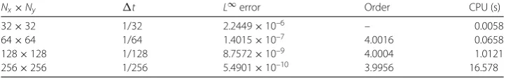
Table 2 Error, order of accuracy, and CPU time with DC4 scheme for Example1
Nx×Ny t L∞error Order CPU (s)
32×32 1/32 2.2449×10⁻⁶ – 0.0058
64×64 1/64 1.4015×10⁻⁷ 4.0016 0.0658
128×128 1/128 8.7572×10⁻⁹ 4.0004 1.0121
256×256 1/256 5.4901×10⁻¹⁰ 3.9956 16.578
Table 3 Error, order of accuracy, and CPU time with DC2, cIIF2, and RK2 schemes for Example2
Nx×Ny×Nz DC2,t= 1/Nx=hx/2π cIIF2,t= 1/Nx=hx/2π RK2,t=h2x/3
L∞error Order CPU (s) L∞error Order CPU (s) L∞error Order CPU (s)
16×16×16 5.50×10⁻⁵ – 0.05 6.95×10⁻³ – 0.04 6.95×10⁻³ – 0.09 32×32×32 3.59×10⁻⁶ 3.94 0.43 1.74×10⁻³ 2.00 0.43 1.74×10⁻³ 2.00 2.06 64×64×64 2.65×10⁻⁷ 3.76 5.93 4.36×10⁻⁴ 2.00 5.95 4.36×10⁻⁴ 2.00 61.9 128×128×128 2.69×10⁻⁸ 3.30 127 1.09×10⁻⁴ 2.00 124 1.09×10⁻⁴ 2.00 2448
a time stept= 1/N2
x to U1and U2. Then we go ahead to simulate the problem using the DC4 scheme with time stept= 1/Nx. The error, order of accuracy, and CPU time for
the DC4 scheme are listed in Table2. We can see that the solution by the DC4 scheme is fourth-order accurate in the temporal and spatial dimensions with time stept= 1/Nx.
The DC4 scheme only triples the CPU time over the DC2 scheme in the meantime.
Example2 Then we consider a similar system in three dimensions on= [0, 2π]2:
∂u ∂t = 0.2
∂2u ∂x2 +
∂2u ∂y2 +
∂2u ∂z2
+ 0.1u (27)
with periodic boundary conditions. The exact solution of this equation is
u=e–0.1tcos(x) +cos(y) +cos(z).
The final computation time ist= 1 at which theL∞error is measured. The time step is chosen ast= 1/Nx. Similar to the two-dimensional case, we list the error, order of
accu-racy, and CPU time for DC2, cIIF2, and RK2 methods in Table3. As shown in Table3, the DC2 scheme achieves higher-order accuracy while requires the same CPU time as cIIF2. The RK2 method requires a much smaller time step and becomes more expensive. Espe-cially for large grid numberN= 128, the computation time is too long to be acceptable. The solution by the DC4 scheme for the three-dimensional case with time stept= 1/Nx
Table 4 Error, order of accuracy, and CPU time with DC4 scheme for Example2
Nx×Ny t L∞error Order CPU (s)
16×16×16 1/16 5.4123×10⁻⁵ – 0.1725
32×32×32 1/32 3.3674×10⁻⁶ 4.0065 1.9944
64×64×64 1/64 2.1022×10⁻⁷ 4.0017 29.632
128×128×128 1/128 1.3136×10⁻⁸ 4.0003 640.60
Figure 1 H0hexagon, stripe, andHπhexagon pattern of CIMA model att= 104for 2D
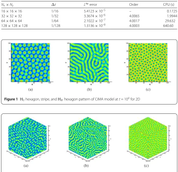
Figure 2 H0hexagon, stripe, andHπhexagon pattern of CIMA model att= 104for 3D
3.2 CIMA model
Example3 Lengyel and Epstein proposed a two-variable kinetic mechanism for CIMA reaction. In this skeleton version, iodide and chlorite play respectively the roles of the activator and the inhibitor:
∂u ∂t =Du∇
2u+ 1 σ
a–u– 4 uv 1 +u2
,
∂v ∂t=Dv∇
2v+b
u– uv 1 +u2
,
(28)
where Du= 1σ, Dv=d, d= 1.07, andσ = 50. We will solve the CIMA model on
two-dimensional case and three-two-dimensional case. The domains on 2D and 3D are chosen as = [0, 100]2and [0, 100]3, respectively. In our computation, we choose the mesh as 64×64 and 64×64×64. Random initial concentration distributions of both species are used. In the simulation the initial condition is taken asu= 10–1rand(· · ·),v= 10–1rand(· · ·), where rand(· · ·) is a random function in Fortran [19].
of values for parametersa,b. The first set (a= 8.8,b= 0.09) leads to an H0hexagon pat-tern as shown in Fig.1(a). The second set (a= 10,b= 0.16) gives rise to a stripe pattern (see Fig.1(b)). The third set (a= 12,b= 0.39) generates an Hπhexagon pattern plotted in
Fig.1(c). Simulations for these three sets of parameters have also been presented in the 3D case. We observe similar patterns by selecting the corresponding parameters, see Fig.2.
4 Concluding remarks
In this paper, we combined the compact FDM in space and the compact IIF method in time to propose a high-order accurate method for solving reaction–diffusion equation. The global accuracy order of this method isO(h4+tr) (r= 2, 3, 4, . . .) and it allows a con-siderable saving in the computation time as the cIIF method. The numerical experiments are conducted to show its superiority over the classical RK method and cIIF method. In the future work we plan to apply the DC scheme for solving the variable coefficients reaction– diffusion problem.
Acknowledgements
The authors would like to thank the referees for their valuable comments and suggestions.
Funding
This work was supported by the National Natural Science Foundation of China (No. 61573008, 61703290), Science Technology on Reliability Environmental Engineering Laboratory (No. 6142A0502020717) and SDUST Research Fund (No. 2014TDJH102).
Availability of data and materials Not applicable.
Competing interests
The authors declare that they have no competing interests.
Authors’ contributions
The authors declare that the study was realized in collaboration with the same responsibility. All authors read and approved the final manuscript.
Author details
1School of Mathematics and Systematic Sciences, Shenyang Normal University, Shenyang, P.R. China.2College of
Mathematics and Systems Science, Shandong University of Science and Technology, Qingdao, P.R. China.3Department of Foreign Language, Shenyang Normal University, Shenyang, P.R. China.
Publisher’s Note
Springer Nature remains neutral with regard to jurisdictional claims in published maps and institutional affiliations.
Received: 6 April 2018 Accepted: 30 July 2018
References
1. Dlamini, P.G., Motsa, S.S., Khumalo, M.: On the comparison between compact finite difference and pseudospectral approaches for solving similarity boundary layer problems. Math. Probl. Eng.2013, Article ID 746489 (2013) 2. Gao, Z., Xie, S.: Fourth-order alternating direction implicit compact finite difference schemes for two-dimensional
Schrödinger equations. Appl. Numer. Math.61, 593–614 (2011)
3. Gierer, A., Meinhardt, H.: A theory of biological pattern formation. Kybernetik12, 30–39 (1972)
4. Gray, P., Scott, S.K.: Autocatalytic reactions in the isothermal, continuous stirred tank reactor: isolas and other forms of multistability. Chem. Eng. Sci.38(1), 29–43 (1983)
5. Gray, R.M.: Toeplitz and circulant matrices. ISL, Tech. Rep., Stanford Univ., Stanford, CA. http://ee-www.stanford.edu/gray/toeplitz.html(2002)
6. Gu, Y., Liao, W., Zhu, J.: An efficient high-order algorithm for solving systems of 3-D reaction–diffusion equations. J. Comput. Appl. Math.155(1), 1–17 (2003)
7. Gurarslan, G., Karahan, H., Alkaya, D., Sari, M., Yasar, M.: Numerical solution of advection–diffusion equation using a sixth-order compact finite difference method. Math. Probl. Eng.2013, Article ID 672936 (2013)
8. Lengyel, I., Epstein, I.R.: Modeling of Turing structures in the chlorite-iodide-malonic acid-starch reaction system. Science251, 650–652 (1991)
10. Liao, W.: A high-order ADI finite difference scheme for a 3D reaction–diffusion equation with Neumann boundary condition. Numer. Methods Partial Differ. Equ.29(3), 778–798 (2013)
11. Nie, Q., Wan, F., Zhang, Y.-T., Liu, X.-F.: Compact integration factor methods in high spatial dimensions. J. Comput. Phys.227, 5238–5255 (2008)
12. Nie, Q., Zhang, Y.-T., Zhao, R.: Efficient semi-implicit schemes for stiff systems. J. Comput. Phys.214, 521–537 (2006) 13. Sambit, D., Liao, W., Gupta, A.: An efficient fourth order low dispersive finite difference scheme for a 2-D acoustic
wave equation. J. Comput. Appl. Math.258, 151–167 (2014)
14. Schnakenberg, J.: Simple chemical reaction systems with limit cycle behavior. J. Theor. Biol.81, 389–400 (1979) 15. Sidje, R.B.: Expokit: software package for computing matrix exponentials. ACM Trans. Math. Softw.24, 130–156 (1998) 16. Wang, D., Zhang, L., Nie, Q.: Array-representation integration factor method for high-dimensional systems. J. Comput.
Phys.258, 585–600 (2014)
17. Wang, Y., Zhang, H.: Higher-order compact finite difference method for systems of reaction–diffusion equations. J. Comput. Appl. Math.233(2), 502–518 (2009)
18. Zhang, R., Liu, J., Zhao, G.: An efficient compact finite difference method for the solution of the Gross–Pitaevskii equation. Adv. Condens. Matter Phys.2015, Article ID 127580 (2015)
19. Zhang, R., Yu, X., Zhu, J., Loula, A.F.D.: Direct discontinuous Galerkin method for nonlinear reaction–diffusion systems in pattern formation. Appl. Math. Model.38, 1612–1621 (2014)